7 Identification based on non-normality of the shocks

7.1 Intuition

In this section, we show that the non-identification of the structural shocks ($\eta_t$) is specific to the Gaussian case. We propose consistent estimation approaches for SVAR in the context of non-Gaussian shocks.

We have seen in what precedes that we cannot identify $B$ based on first and second moments only. Since a Gaussian distribution is perfectly determined by the first two moments, it comes that one cannot achieve identification when the structural shocks are Gaussian. That is, even if we observe an infinite number of i.i.d. $B \eta_t$, we cannot recover $B$ is the $\eta_t$’s are Gaussian.

Indeed, if $\eta_t \sim \mathcal{N}(0,Id)$, then the distribution of $\varepsilon_t \equiv B \eta_t$ is $\mathcal{N}(0,BB')$. Hence $\Omega = B B'$ is observed (in the population), but for any orthogonal matrix $Q$ (i.e. $QQ'=Id$), we also have $BQ \eta_t \sim \mathcal{N}(0,\Omega)$.

To illustrate, consider the following bivariate Gaussian situations, with $\Theta_1=0$):

$\left[\begin{array}{c}\eta_{1,t}\\ \eta_{2,t}\end{array}\right]\sim \mathcal{N}(0,Id)$, with $B = \left[\begin{array}{cc} 1 & 2 \\ -1 & 1 \end{array}\right]$ and $Q = \left[\begin{array}{cc} \cos(\pi/3) & -\sin(\pi/3) \\ \sin(\pi/3) & \cos(\pi/3) \end{array}\right]$ (rotation).

Figure 7.1 shows that the distributions of $B \eta_t$ and of $BQ\eta_t$ are identical. However, the impulse response functions associated with one of the other impulse matrix ($B$ or $BQ$) are different. This is illustrated by Figure 7.2, that shows the IRFs associated with two identical models (defined by Eq. (1.5)), the only difference being the impulse matrix ($B$ or $BQ$).

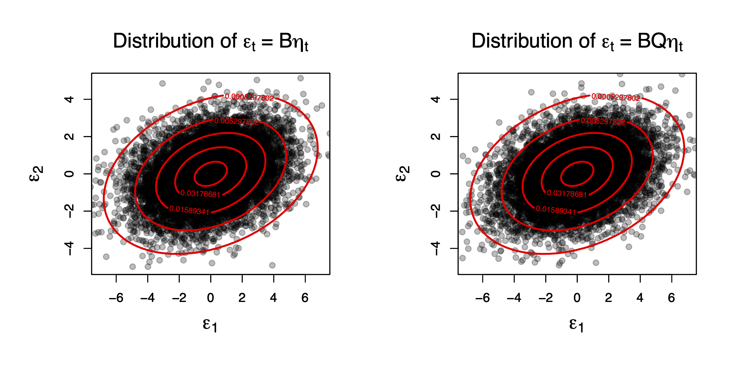
$This figure compares the distributions of two Gaussian bivariate vectors, $B \eta_t$ and $BQ\eta_t$, where $\eta_{t} \sim \mathcal{N}(0,Id)$ (therefore $\eta_{1,t}$ and $\eta_{2,t}$ are independent), and $Q$ is an orthogonal matrix.$

Figure 7.1: This figure compares the distributions of two Gaussian bivariate vectors, $B \eta_t$ and $BQ\eta_t$, where $\eta_{t} \sim \mathcal{N}(0,Id)$ (therefore $\eta_{1,t}$ and $\eta_{2,t}$ are independent), and $Q$ is an orthogonal matrix.

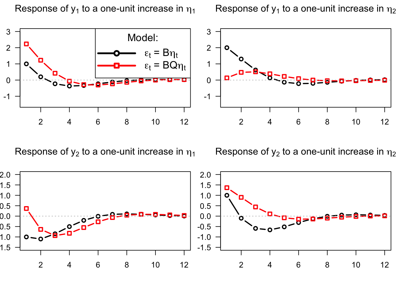
This figure shows that the impulse response functions associated with an impulse matrix equal to $B$ (black line) or $BQ$ (red line) are different (even if $BB'=BQ(BQ)'$).

Figure 7.2: This figure shows that the impulse response functions associated with an impulse matrix equal to $B$ (black line) or $BQ$ (red line) are different (even if $BB'=BQ(BQ)'$).

Hence, in the Gaussian case, external restrictions (economic hypotheses) are needed to identify $B$ (see previous sections). But such restrictions may not be necessary if the structural shocks are not Gaussian. That is, the identification problem is very specific to normally-distributed $\eta_t$’s (Rigobon (2003), Normandin and Phaneuf (2004), Lanne and Lütkepohl (2008)).

To better see why this can be the case, consider again a bivariate vector of independent structural shocks ($\eta_{1,t}$ and $\eta_{2,t}$) but, now, assume that one of them is not Gaussian any more. Specifically, assume that $\eta_{2,t}$ is drawn from a Student distribution with 5 degrees of freedom: $\eta_{1,t} \sim \mathcal{N}(0,1)$, $\eta_{2,t} \sim t(5)$, $B = \left[\begin{array}{cc} 1 & 2 \\ -1 & 1 \end{array}\right]$ and $Q = \left[\begin{array}{cc} \cos(\pi/3) & -\sin(\pi/3) \\ \sin(\pi/3) & \cos(\pi/3) \end{array}\right]$.

Figure 7.3 shows that, in this case, $B \eta_t$ and $BQ\eta_t$ do not have the same distribution any more (in spite of the fact that, in both cases, we have $\mathbb{V}ar(\varepsilon_t)=BB'$). This opens the door to the identification of the impulse matrix ($BQ$) in the non-Gaussian case.

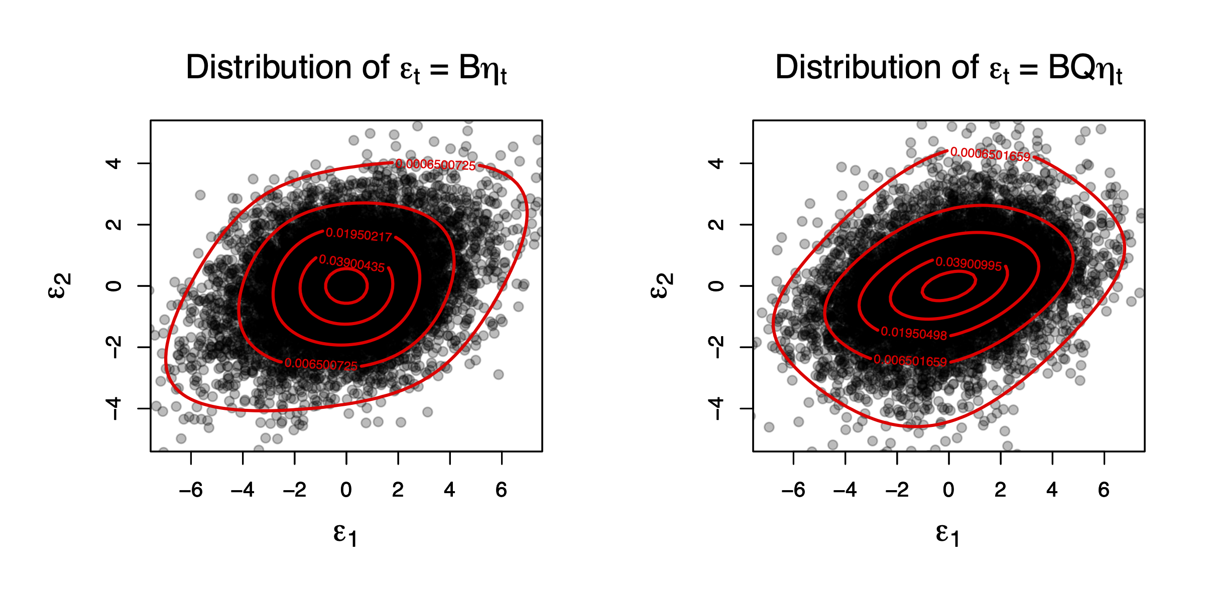
$This figure compares the distributions of two Gaussian bivariate vectors, $B \eta_t$ and $BQ\eta_t$, where $\eta_t{1,t} \sim \mathcal{N}(0,1)$, $\eta_t{2,t} \sim t(5)$, and $Q$ is an orthogonal matrix.$

Figure 7.3: This figure compares the distributions of two Gaussian bivariate vectors, $B \eta_t$ and $BQ\eta_t$, where $\eta_t{1,t} \sim \mathcal{N}(0,1)$, $\eta_t{2,t} \sim t(5)$, and $Q$ is an orthogonal matrix.

7.2 Independent Component Analysis (ICA)

The exercise that consists in identifying non-Gaussian independent shocks out of linear combinations of these shocks is a well-known problem of the signal-processing literature, called independent component analysis (ICA). Let us denote by $C$ the matrix that is such that $C = \Omega^{-1/2}B$, where $\Omega^{1/2}$ results from the Cholesky decomposition of $\Omega = BB'$ (implying, $\Omega^{1/2}{\Omega^{1/2}}'=\Omega$). It is easy to check that $C$ is an orthogonal matrix (and we have $B = \Omega^{1/2}C$).

The classical ICA problem is as follows: Find $C$ such that $\varepsilon_t = C \eta_t$ (or $\eta_t = C'\varepsilon_t$) given that:⁷

We observe the $\varepsilon_t$’s,
The components of $\eta_t$ are independent,
$CC'=Id$ (i.e., $C$ is orthogonal).

Figure 7.4 represents again some bivariate distributions. The black (red) lines correspond to the distributions of $\eta_t$ ($C\eta_t$). It is important to note that the two components of vector $C \eta_t$ are not independent (contrary to those of $\eta_t$).

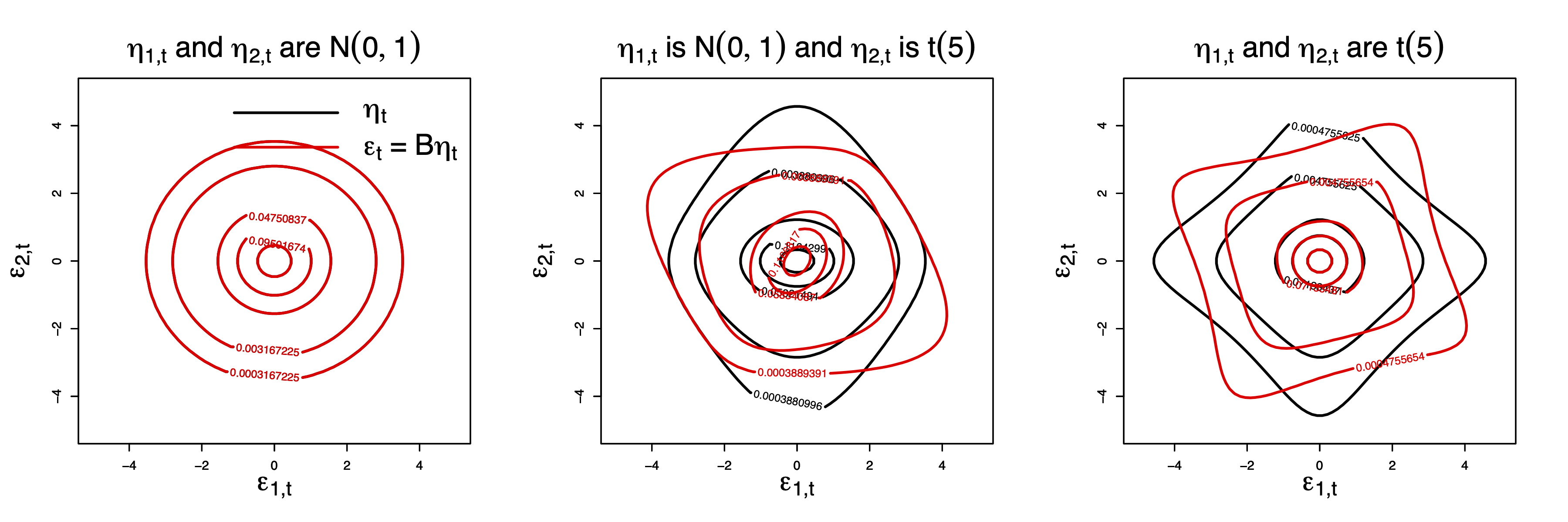
$The three plots represent the bivariate distributions of $\eta_t$ (black) and of $C\eta_t$ (red), where the two components of $\eta_t$ are independent, of unit variance, and $C$ is orthogonal. Hence, for each of the three plots, $\mathbb{V}ar(C\eta_t)=Id$.$

Figure 7.4: The three plots represent the bivariate distributions of $\eta_t$ (black) and of $C\eta_t$ (red), where the two components of $\eta_t$ are independent, of unit variance, and $C$ is orthogonal. Hence, for each of the three plots, $\mathbb{V}ar(C\eta_t)=Id$.

In all cases, we have $\mathbb{V}ar(\varepsilon_t)=\mathbb{V}ar(\eta_t)=Id$. But the two components of $\varepsilon_t$ are not independent. For instance, in the last two cases, we have $\mathbb{E}(\varepsilon_{2,t}|\varepsilon_{1,t}>4)<0$ (whereas $\mathbb{E}(\eta_{2,t}|\eta_{1,t}>4)=0$). The objective of ICA is to rotate $\varepsilon_t$ to retrieve independent components ($\eta_t$).

Hypothesis 7.1 Process $\eta_t$ satisfies:

The $\eta_t$’s are i.i.d. (across time) with $\mathbb{E}(\eta_t) = 0$ and $\mathbb{V}ar(\eta_t) = Id.$
The components $\eta_{1,t}, \ldots, \eta_{n,t}$ are mutually independent. iii We have \[ \varepsilon_t = C_0 \eta_t, \] with $\mathbb{V}ar(\varepsilon_t) = Id$ (i.e., $C_0$ is orthogonal).

Theorem 7.1 (Eriksson, Koivunen (2004)) If Hypothesis 7.1 is satisfied and if at most one of the components of $\eta$ is Gaussian, then matrix $C_0$ is identifiable up to the post multiplication by $DP$, where $P$ is a permutation matrix and $D$ is a diagonal matrix whose diagonal entries are 1 or $-1$.}

7.3 Pseudo-Maximum Likelihood (PML) approach

Hence, non-normal structural shocks are identifiable. But how to estimate them based on observations of the $\varepsilon_t$’s? Gouriéroux, Monfort, and Renne (2017) have proposed a Pseudo-Maximum Likelihood (PML) approach. This approach consists in maximizing a so-called pseudo log-likelihood function, based on a set of p.d.f. $g_i (\eta_i), i=1,\ldots,n$ (that may be different from the true p.d.f. of the $\eta_{i,t}$’s): \[\begin{equation} \log \mathcal{L}_T (C) = \sum^T_{t=1} \sum^n_{i=1} \log g_i (c'_i \varepsilon_t),\tag{7.1} \end{equation}\] where $c_i$ is the $i^{th}$ column of matrix $C$ (or $c'_i$ is the $i^{th}$ row of $C^{-1}$ since $C^{-1}=C'$).

The log-likelihood function (7.1) is computed as if the errors $\eta_{i,t}$ had the pdf $g_i (\eta_i)$. The PML estimator of matrix $C$ maximizes the pseudo log-likelihood function: \[\begin{equation} \widehat{C_T} = \arg \max_C \sum^T_{t=1} \sum^n_{i=1} \log g_i (c'_i \varepsilon_t),\tag{7.2} \end{equation}\]

The restrictions $C'C = Id$ can be eliminated by parameterizing $C$ in such a way that, whatever the considered parameters, $C$ is orthogonal.⁸ Gouriéroux, Monfort, and Renne (2017) propose to use, for that, the Cayley’s representation: any orthogonal matrix with no eigenvalue equal to $-1$ can be written as \[\begin{equation} C(A) = (Id+A) (Id-A)^{-1}, \end{equation}\] where $A$ is a skew symmetric (or antisymmetric) matrix, such that $A'=-A$. There is a one-to-one relationship with $A$, since: \[\begin{equation} A = (C(A)+Id)^{-1} (C(A)-Id). \end{equation}\]

Hence, the PML estimator of matrix $C$ is obtained as $\widehat{C_T} = C(\hat{A}_T),$ where: \[\begin{equation} \hat{A}_T = \arg \max_{a_{i,j}, i>j} \sum^T_{t=1} \sum^n_{i=1} \log g_i [c_i (A)' \varepsilon_t].\tag{7.3} \end{equation}\]

Under assumptions on the $g_i$ functions (excluding the Gaussian distributions), Gouriéroux, Monfort, and Renne (2017) derive the asymptotic properties of the PML estimator. Specifically, the PML estimator $\widehat{C_T}$ of $C_0$ is consistent (in $\mathcal{P}_0$, the set of matrices obtained by permutation and sign change of the columns of $C_0$) and asymptotically normal, with speed of convergence $1/\sqrt{T}$.

The asymptotic variance-covariance matrix of $vec \sqrt{T} (\widehat{C_T} - C_0)$ is $A^{-1} \left[\begin{array}{cc} \Gamma & 0 \\ 0 & 0 \end{array} \right] (A')^{-1}$, where matrices $A$ and $\Gamma$ are detailed in Gouriéroux, Monfort, and Renne (2017).

Note that the potential misspecification of pseudo-distributions $g_i$ has no effect on the consistency of these specific PML estimators.

Table 7.1 reports usual p.d.f. and their derivatives. (The latter are needed to compute the asymptotic variance-covariance matrix of $vec \sqrt{T} (\widehat{C_T} - C_0)$.)

Table 7.1: This table reports usual p.d.f. and their derivatives.
	$\log g(x)$	$\dfrac{d \log g(x)}{d x}$	$\dfrac{d^2 \log g(x)}{d x^2}$
Gaussian	$cst - x^2/2$	$-x$	$-1$
Student $t(\nu>4)$	$-\dfrac{1-\nu}{2}\log\left( 1 +\dfrac{x^2}{\nu-2} \right)$	$-\dfrac{x(1+\nu)}{\nu - 2 + x^2}$	$- (1+\nu) \dfrac{\nu - 2 - x^2}{\nu - 2 + x^2}$
Hyperbolic secant	$cst - \log\left( \cosh\left\{\dfrac{\pi}{2}x\right\} \right)$	$-\dfrac{\pi}{2} anh\left(\dfrac{\pi}{2}x\right)$	$-\left(\dfrac{\pi}{2}\dfrac{1}{\cosh\left(\dfrac{\pi}{2}x\right)}\right)^2$
Subgaussian	$cst + \pi x^2 + \log \left(\cosh\left\{\dfrac{\pi}{2}x\right\}\right)$	$2\pi x+\dfrac{\pi}{2}\tanh\left(x \dfrac{\pi}{2}\right)$	$2\pi +\left(\dfrac{\pi}{2}\dfrac{1}{\cosh\left(\dfrac{\pi}{2}x\right)}\right)^2$

Example 7.1 (Non-Gaussian monetary-policy shocks) We apply the PML-ICA approach on U.S. data coerving the period 1959:IV to 2015:I at the quarterly frequency ($T=224$). We consider three dependent variables: inflation ($\pi_t$), economic activity ($z_t$, the output gap) and the nominal short-term interest rate ($r_t$). Changes in the log of oil prices are added as an exogenous variable ($x_t$).

library(IdSS)
First.date <- "1959-04-01"
Last.date  <- "2015-01-01"
data <- US3var
data <- data[(data$Date>=First.date)&(data$Date<=Last.date),]
Y <- as.matrix(data[c("infl","y.gdp.gap","r")])
names.var <- c("inflation","real activity","short-term rate")
T <- dim(Y)[1]
n <- dim(Y)[2]

Let us denote by $W_t$ the set of information made of the past values of $y_t= [\pi_t,z_t,r_t]$, that is $\{y_{t-1},y_{t-2},\dots\}$, and of exogenous variables $\{x_{t},x_{t-1},\dots\}$. The reduced-form VAR model reads: \[ y_t = \underbrace{\mu + \sum_{i=1}^{p} \Phi_i y_{t-i} + \Theta x_t}_{a(W_t;\theta)} + u_t \] where the $u_t$’s are assumed to be serially independent, with zero mean and variance-covariance matrix $\Omega$.

Matrices $\mu$, $\Phi_i$, $\Theta$ and $\Omega$ are consistently estimated by OLS. Jarque-Bera tests support the hypothesis of non-normality for all residuals.

nb.lags <- 6 # number of lags used in the VAR model
X <- NULL
for(i in 1:nb.lags){
  lagged.Y <- rbind(matrix(NaN,i,n),Y[1:(T-i),])
  X <- cbind(X,lagged.Y)}
X <- cbind(X,data$commo) # add exogenous variables
Phi <- matrix(0,n,n*nb.lags);mu <- rep(0,n)
effect.commo <- rep(0,n)
U <- NULL # Eta is the matrix of OLS residuals
for(i in 1:n){
  eq <- lm(Y[,i] ~ X)
  Phi[i,] <- eq$coef[2:(dim(Phi)[2]+1)]
  mu[i] <- eq$coef[1]
  U <- cbind(U,eq$residuals)
  effect.commo[i] <- eq$coef[length(eq$coef)]
}
Omega <- var(U) # Covariance matrix of the OLS residuals.
Omeg12 <- t(chol(Omega)) # Cholesky matrix associated with Omega (lower triang.)
Eps <- U %*% t(solve(Omeg12)) # Recover associated structural shocks

We want to estimate the orthogonal matrix $C$ such that $u_t=\Omega^{1/2}C \eta_t$, where

$\Omega^{1/2}$ results from the Cholesky decomposition of $\Omega$ and
the components of $\eta_t$ are independent, zero-mean with unit variance.

The PML approach is applied on standardized VAR residuals given by: \[ \hat\varepsilon_t = \hat\Omega^{-1/2}_T\underbrace{[y_t - a(W_t;\hat\theta_T)]}_{\mbox{VAR residuals}}. \] By construction of $\hat\Omega^{-1/2}_T$, it comes that the covariance matrix of these residuals is $Id$.

The pseudo density functions are distinct and asymmetric mixtures of Gaussian distributions.

distri <- list(
  type=c("mixt.gaussian","mixt.gaussian","mixt.gaussian"),
  df=c(NaN,NaN,NaN),
  p=c(0.5,.5,.5),mu=c(.1,.1,.1),sigma=c(.5,.7,1.3))
AA.0 <- c(0,0,0)
res.optim <- optim(AA.0,func.2.minimize,
                   Y = Eps, distri = distri,
                   gr = d.func.2.minimize,
                   method="Nelder-Mead",
                   control=list(trace=FALSE,maxit=1000))
AA.0 <- res.optim$par
res.optim <- optim(AA.0,func.2.minimize,d.func.2.minimize,
                   Y = Eps, distri = distri,
                   method="BFGS",
                   control=list(trace=FALSE))
AA.est <- res.optim$par
n <- ncol(Y)
M <- make.M(n)
A.est <- matrix(M %*% AA.est,n,n)
C.PML <- (diag(n) + A.est) %*% solve(diag(n) - A.est)
eta.PML <- Eps %*% C.PML # eta.PML are the ICA-estimated structural shocks

# Compute asymptotic covariance matrix of C.PML:
V <- make.Asympt.Cov.delta(eta.PML,distri,C.PML)
param <- c(C.PML)
st.dev <- sqrt(diag(V))
t.stat <- c(C.PML)/sqrt(diag(V))
cbind(param,st.dev,t.stat) # print results of PML estimation

##             param      st.dev      t.stat
##  [1,]  0.94417705 0.040848382  23.1141845
##  [2,] -0.32711569 0.118802653  -2.7534376
##  [3,]  0.03905164 0.074172945   0.5264944
##  [4,]  0.32070293 0.119270893   2.6888616
##  [5,]  0.93977707 0.041629110  22.5749976
##  [6,]  0.11818924 0.060821400   1.9432179
##  [7,] -0.07536139 0.071980455  -1.0469702
##  [8,] -0.09906759 0.062185577  -1.5930959
##  [9,]  0.99222290 0.007785691 127.4418551

(Note: it is always useful to combine two optimization algorithms, such as Nelder-Mead and BFGS.)

We would obtain close results by neglecting commodity prices. In that case, one can simply use the function estim.SVAR.ICA of the IdSS package. Let us compare the $C$ matrix obtained in the two cases (with or without commodity prices):

ICA.res.no.commo <- estim.SVAR.ICA(Y,distri = distri,p=6)
round(cbind(ICA.res.no.commo$C.PML,NaN,C.PML),3)

##        [,1]  [,2]   [,3] [,4]   [,5]  [,6]   [,7]
## [1,]  0.956 0.287 -0.059  NaN  0.944 0.321 -0.075
## [2,] -0.292 0.950 -0.108  NaN -0.327 0.940 -0.099
## [3,]  0.025 0.121  0.992  NaN  0.039 0.118  0.992

Once $C$ has been estimated, it remains to label the resulting structural shocks (components of $\eta_{t}$). Postulated shocks are monetary-policy, supply, and demand shocks. This labelling can be based on the following considerations:

Contractionary monetary-policy shocks have a negative impact on real activity and on inflation.
Supply shock have influences of opposite signs on economic activity and on inflation.
Demand shock have influences of same signs on economic activity and on inflation.

Let us compute the IRFs associated with the three structural shocks. (For the sake of comparison, the first line of plots shows the IRFs to a monetary-policy shock obtained from a Cholesky-based approach where the short-term rate is ordered last.)

IRF.Chol <- array(NaN,c(n,41,n))
IRF.ICA  <- array(NaN,c(n,41,n))
PHI <- list();for(i in 1:nb.lags){PHI[[i]]<-array(Phi,c(3,3,nb.lags))[,,i]}
for(jjjj in 1:n){
  u.shock <- rep(0,n)
  u.shock[jjjj] <- 1
  IRF.Chol[,,jjjj] <- 
    t(simul.VAR(c=rep(0,3),Phi=PHI,B=Omeg12,nb.sim=41,
                y0.star=rep(0,3*nb.lags),indic.IRF = 1,u.shock = u.shock))
  IRF.ICA[,,jjjj]  <- 
    t(simul.VAR(c=rep(0,3),Phi=PHI,B=Omeg12%*%C.PML,nb.sim=41,
                y0.star=rep(0,3*nb.lags),indic.IRF = 1,u.shock = u.shock))
}

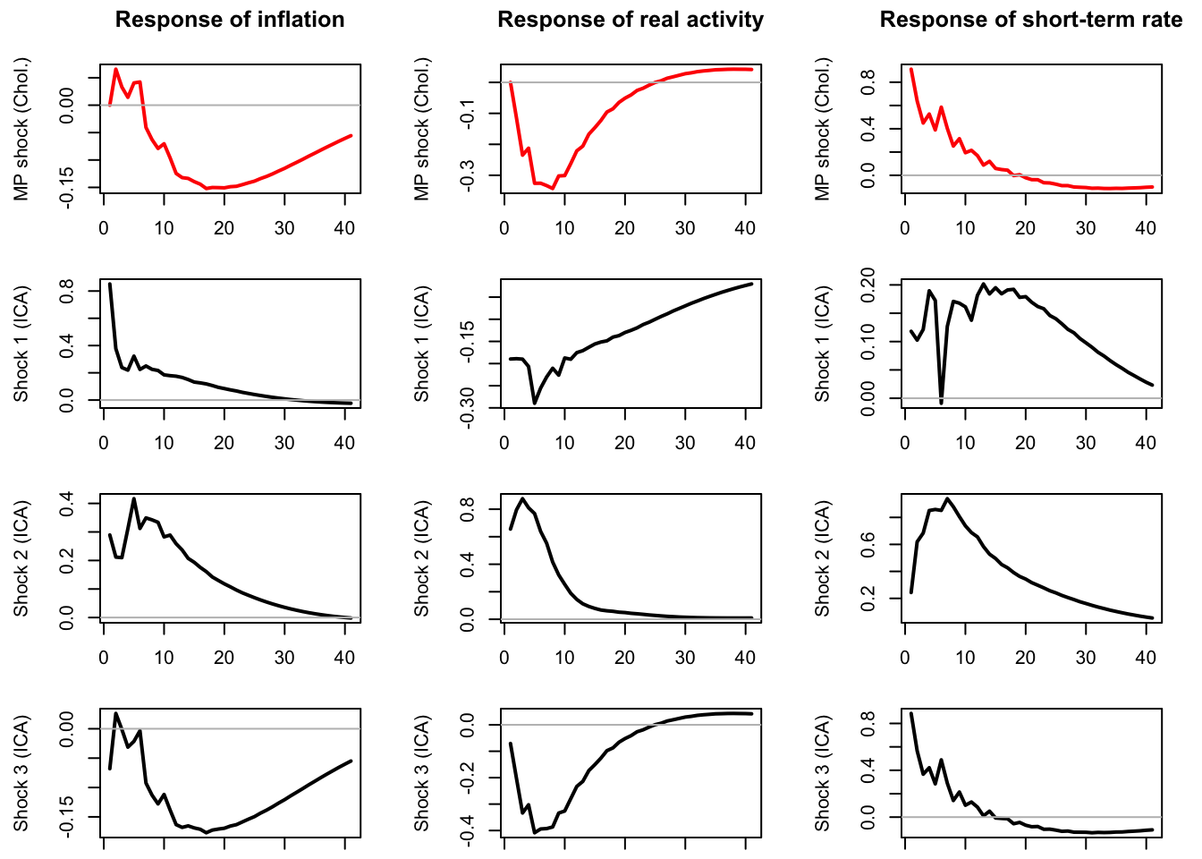
The first row of plots shows the responses of the three endogenous variables to the monetary policy shock in the context of a Cholesky-idendtified SVAR (ordering: inflation, output gap, interest rate). The next three rows of plots show the repsonses of the endogenous variables to the three structural shocks identified by ICA. The last one (Shock 3) is close to the Cholesky-identified monetary policy shock.

Figure 7.5: The first row of plots shows the responses of the three endogenous variables to the monetary policy shock in the context of a Cholesky-idendtified SVAR (ordering: inflation, output gap, interest rate). The next three rows of plots show the repsonses of the endogenous variables to the three structural shocks identified by ICA. The last one (Shock 3) is close to the Cholesky-identified monetary policy shock.

According to Figure 7.5, Shock 1 is a supply shock, Shock 2 is a demand shock, and Shock 3 is a monetary-policy shock. Note that Shock 3 is close to the one resulting from the Cholesky approach.

7.4 Relation with the Heteroskedasticity Identification

In some cases, where the $\varepsilon_t$’s are heteroskedastic, the $B$ matrix can be identified (Rigobon (2003), Lanne, Lütkepohl, and Maciejowska (2010)).

Consider the case where we still have $\varepsilon_t = B \eta_t$ but where $\eta_t$’s variance conditionally depends on a regime $s_t \in \{1,\dots,M\}$. That is: \[ \mathbb{V}ar(\eta_{k,t}|s_t) = \lambda_{s_t,k} \quad \mbox{for } k \in \{1,\dots,n\} \]

Denoting by $\Lambda_i$ the diagonal matrix whose diagonal entries are the $\lambda_{i,k}$’s, it comes that: \[ \mathbb{V}ar(\eta_{t}|s_t) = \Lambda_{s_t},\quad \mbox{and}\quad \mathbb{V}ar(\varepsilon_{t}|s_t) = B\Lambda_{s_t}B'. \]

Without loss of generality, it can be assumed that $\Lambda_1=Id$.

In this context, $B$ is identified, apart from sign reversal of its columns if for all $k \ne j \in \{1,\dots,n\}$, there is a regime $i$ s.t. $\lambda_{i,k} \ne \lambda_{i,j}$. (Prop.1 in Lanne, Lütkepohl, and Maciejowska (2010)).

Bivariate regime case ($M=2$): $B$ identified if the $\lambda_{2,k}$’s are all different. That is, identification is ensured if “there is sufficient heterogeneity in the volatility changes” (Lütkepohl and Netšunajev (2017)).

If the regimes $s_t$ are exogenous and serially independent, then this situation is consistent with the “non-Gaussian” situation described above.

6 Forecast error variance maximization

8 Local projection methods

	\(\log g(x)\)	\(\dfrac{d \log g(x)}{d x}\)	\(\dfrac{d^2 \log g(x)}{d x^2}\)
Gaussian	\(cst - x^2/2\)	\(-x\)	\(-1\)
Student \(t(\nu>4)\)	\(-\dfrac{1-\nu}{2}\log\left( 1 +\dfrac{x^2}{\nu-2} \right)\)	\(-\dfrac{x(1+\nu)}{\nu - 2 + x^2}\)	\(- (1+\nu) \dfrac{\nu - 2 - x^2}{\nu - 2 + x^2}\)
Hyperbolic secant	\(cst - \log\left( \cosh\left\{\dfrac{\pi}{2}x\right\} \right)\)	\(-\dfrac{\pi}{2} anh\left(\dfrac{\pi}{2}x\right)\)	\(-\left(\dfrac{\pi}{2}\dfrac{1}{\cosh\left(\dfrac{\pi}{2}x\right)}\right)^2\)
Subgaussian	\(cst + \pi x^2 + \log \left(\cosh\left\{\dfrac{\pi}{2}x\right\}\right)\)	\(2\pi x+\dfrac{\pi}{2}\tanh\left(x \dfrac{\pi}{2}\right)\)	\(2\pi +\left(\dfrac{\pi}{2}\dfrac{1}{\cosh\left(\dfrac{\pi}{2}x\right)}\right)^2\)

References

The \(\varepsilon_t\)’s that we consider here are standardized VAR residuals, obtained by pre-multiplying the actual VAR residuals by \(\Omega^{-1/2}\).↩︎
Jarocinski (2021) develops a ML approach that does not necessitates to parameterize the space of orthogonal matrices as he does not proceed under the assumption that \(C'C\) is orthogonal.↩︎