11 Appendix

11.1 Definitions and statistical results

Definition 11.1 (Covariance stationarity) The process \(y_t\) is covariance stationary —or weakly stationary— if, for all \(t\) and \(j\), \[ \mathbb{E}(y_t) = \mu \quad \mbox{and} \quad \mathbb{E}\{(y_t - \mu)(y_{t-j} - \mu)\} = \gamma_j. \]

Definition 11.2 (Likelihood Ratio test statistics) The likelihood ratio associated to a restriction of the form \(H_0: h({\boldsymbol\theta})=0\) (where \(h({\boldsymbol\theta})\) is a \(r\)-dimensional vector) is given by: \[ LR = \frac{\mathcal{L}_R(\boldsymbol\theta;\mathbf{y})}{\mathcal{L}_U(\boldsymbol\theta;\mathbf{y})} \quad (\in [0,1]), \] where \(\mathcal{L}_R\) (respectively \(\mathcal{L}_U\)) is the likelihood function that imposes (resp. that does not impose) the restriction. The likelihood ratio test statistic is given by \(-2\log(LR)\), that is: \[ \boxed{\xi^{LR}= 2 (\log\mathcal{L}_U(\boldsymbol\theta;\mathbf{y})-\log\mathcal{L}_R(\boldsymbol\theta;\mathbf{y})).} \] Under regularity assumptions and under the null hypothesis, the test statistic follows a chi-square distribution with \(r\) degrees of freedom (see Table 11.3).

Proposition 11.1 (p.d.f. of a multivariate Gaussian variable) If \(Y \sim \mathcal{N}(\mu,\Omega)\) and if \(Y\) is a \(n\)-dimensional vector, then the density function of \(Y\) is: \[ \frac{1}{(2 \pi)^{n/2}|\Omega|^{1/2}}\exp\left[-\frac{1}{2}\left(Y-\mu\right)'\Omega^{-1}\left(Y-\mu\right)\right]. \]

11.2 Estimation of VARMA models

Section 1.4 discusses the estimation of VAR models and shows that standard VAR models can be esitmated by running OLS regressions.

If there is an MA component (i.e., if we consider a VARMA model), then OLS regressions yield biased estimates (even for asymptotically large samples). Assume for instance that \(y_t\) follows a VARMA(1,1) model: \[ y_{i,t} = \phi_i y_{t-1} + \varepsilon_{i,t}, \] where \(\phi_i\) is the \(i^{th}\) row of \(\Phi_1\), and where \(\varepsilon_{i,t}\) is a linear combination of \(\eta_t\) and \(\eta_{t-1}\). Since \(y_{t-1}\) (the regressor) is correlated to \(\eta_{t-1}\), it is also correlated to \(\varepsilon_{i,t}\). The OLS regression of \(y_{i,t}\) on \(y_{t-1}\) yields a biased estimator of \(\phi_i\) (see Figure 11.1). Hence, SVARMA models cannot be consistently estimated by simple OLS regressions (contrary to VAR models, as we will see in the next section); instrumental-variable approaches can be employed to estimate SVARMA models (using past values of \(y_t\) as instruments, see, e.g., Gouriéroux, Monfort, and Renne (2020)).

N <- 1000 # number of replications
T <- 100 # sample length
phi <- .8 # autoregressive parameter
sigma <- 1
par(mfrow=c(1,2))
for(theta in c(0,-0.4)){
  all.y <- matrix(0,1,N)
  y     <- all.y
  eta_1 <- rnorm(N)
  for(t in 1:(T+1)){
    eta <- rnorm(N)
    y <- phi * y + sigma * eta + theta * sigma * eta_1
    all.y <- rbind(all.y,y)
    eta_1 <- eta
  }
  all.y_1 <- all.y[1:T,]
  all.y   <- all.y[2:(T+1),]
  XX_1 <- 1/apply(all.y_1 * all.y_1,2,sum)
  XY   <- apply(all.y_1 * all.y,2,sum)
  phi.est.OLS <- XX_1 * XY
  plot(density(phi.est.OLS),xlab="OLS estimate of phi",ylab="",
       main=paste("theta = ",theta,sep=""))
  abline(v=phi,col="red",lwd=2)}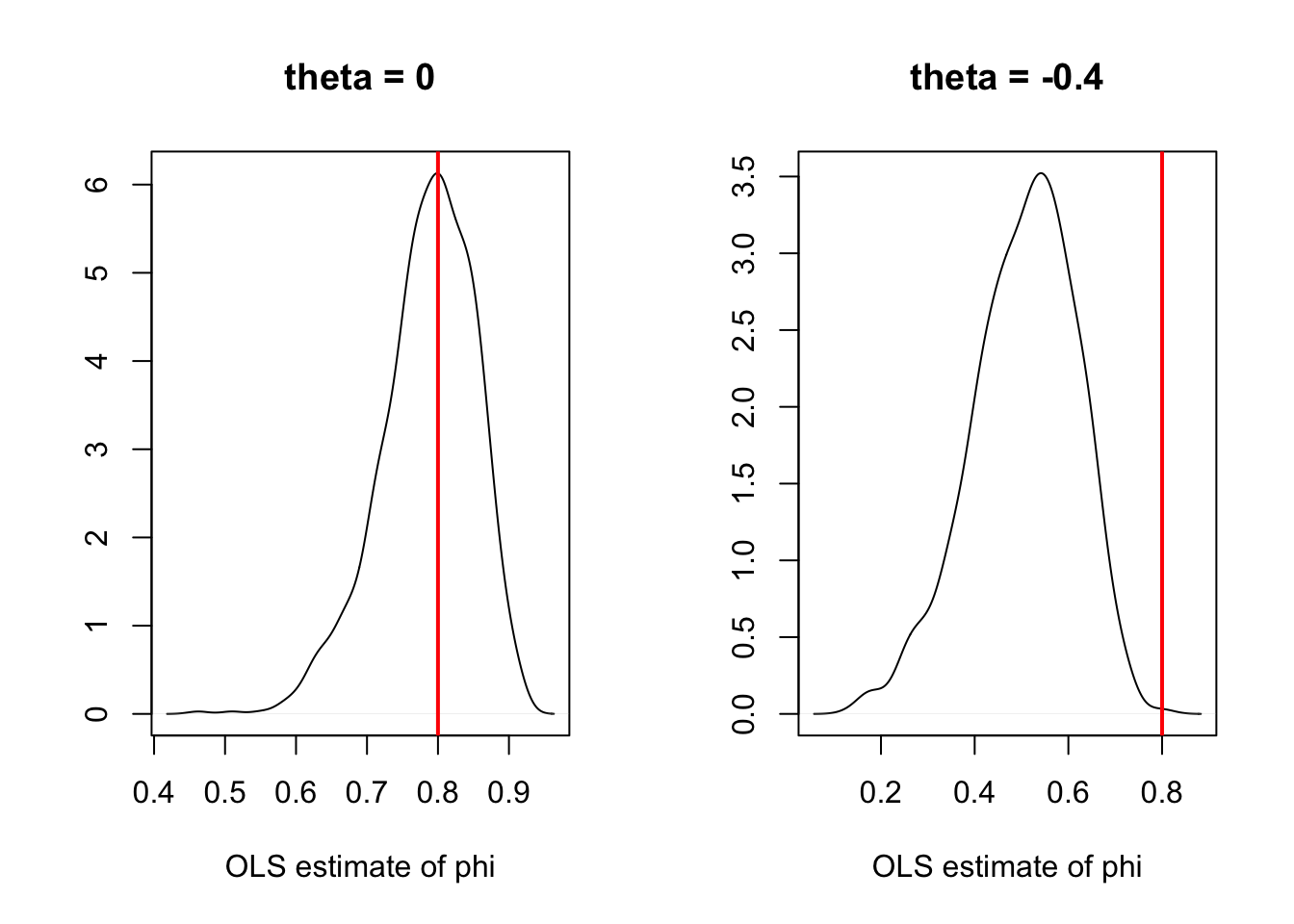

Figure 11.1: Illustration of the bias obtained when estimating the auto-regressive parameters of an ARMA process by (standard) OLS.

11.3 Proofs

Proof of Proposition 1.2

Proof. Using Proposition 11.1, we obtain that, conditionally on \(x_1\), the log-likelihood is given by \[\begin{eqnarray*} \log\mathcal{L}(Y_{T};\theta) & = & -(Tn/2)\log(2\pi)+(T/2)\log\left|\Omega^{-1}\right|\\ & & -\frac{1}{2}\sum_{t=1}^{T}\left[\left(y_{t}-\Pi'x_{t}\right)'\Omega^{-1}\left(y_{t}-\Pi'x_{t}\right)\right]. \end{eqnarray*}\] Let’s rewrite the last term of the log-likelihood: \[\begin{eqnarray*} \sum_{t=1}^{T}\left[\left(y_{t}-\Pi'x_{t}\right)'\Omega^{-1}\left(y_{t}-\Pi'x_{t}\right)\right] & =\\ \sum_{t=1}^{T}\left[\left(y_{t}-\hat{\Pi}'x_{t}+\hat{\Pi}'x_{t}-\Pi'x_{t}\right)'\Omega^{-1}\left(y_{t}-\hat{\Pi}'x_{t}+\hat{\Pi}'x_{t}-\Pi'x_{t}\right)\right] & =\\ \sum_{t=1}^{T}\left[\left(\hat{\varepsilon}_{t}+(\hat{\Pi}-\Pi)'x_{t}\right)'\Omega^{-1}\left(\hat{\varepsilon}_{t}+(\hat{\Pi}-\Pi)'x_{t}\right)\right], \end{eqnarray*}\] where the \(j^{th}\) element of the \((n\times1)\) vector \(\hat{\varepsilon}_{t}\) is the sample residual, for observation \(t\), from an OLS regression of \(y_{j,t}\) on \(x_{t}\). Expanding the previous equation, we get: \[\begin{eqnarray*} &&\sum_{t=1}^{T}\left[\left(y_{t}-\Pi'x_{t}\right)'\Omega^{-1}\left(y_{t}-\Pi'x_{t}\right)\right] = \sum_{t=1}^{T}\hat{\varepsilon}_{t}'\Omega^{-1}\hat{\varepsilon}_{t}\\ &&+2\sum_{t=1}^{T}\hat{\varepsilon}_{t}'\Omega^{-1}(\hat{\Pi}-\Pi)'x_{t}+\sum_{t=1}^{T}x'_{t}(\hat{\Pi}-\Pi)\Omega^{-1}(\hat{\Pi}-\Pi)'x_{t}. \end{eqnarray*}\] Let’s apply the trace operator on the second term (that is a scalar): \[\begin{eqnarray*} \sum_{t=1}^{T}\hat{\varepsilon}_{t}'\Omega^{-1}(\hat{\Pi}-\Pi)'x_{t} & = & Tr\left(\sum_{t=1}^{T}\hat{\varepsilon}_{t}'\Omega^{-1}(\hat{\Pi}-\Pi)'x_{t}\right)\\ = Tr\left(\sum_{t=1}^{T}\Omega^{-1}(\hat{\Pi}-\Pi)'x_{t}\hat{\varepsilon}_{t}'\right) & = & Tr\left(\Omega^{-1}(\hat{\Pi}-\Pi)'\sum_{t=1}^{T}x_{t}\hat{\varepsilon}_{t}'\right). \end{eqnarray*}\] Given that, by construction (property of OLS estimates), the sample residuals are orthogonal to the explanatory variables, this term is zero. Introducing \(\tilde{x}_{t}=(\hat{\Pi}-\Pi)'x_{t}\), we have \[\begin{eqnarray*} \sum_{t=1}^{T}\left[\left(y_{t}-\Pi'x_{t}\right)'\Omega^{-1}\left(y_{t}-\Pi'x_{t}\right)\right] =\sum_{t=1}^{T}\hat{\varepsilon}_{t}'\Omega^{-1}\hat{\varepsilon}_{t}+\sum_{t=1}^{T}\tilde{x}'_{t}\Omega^{-1}\tilde{x}_{t}. \end{eqnarray*}\] Since \(\Omega\) is a positive definite matrix, \(\Omega^{-1}\) is as well. Consequently, the smallest value that the last term can take is obtained for \(\tilde{x}_{t}=0\), i.e. when \(\Pi=\hat{\Pi}.\)

The MLE of \(\Omega\) is the matrix \(\hat{\Omega}\) that maximizes \(\Omega\overset{\ell}{\rightarrow}L(Y_{T};\hat{\Pi},\Omega)\). We have: \[\begin{eqnarray*} \log\mathcal{L}(Y_{T};\hat{\Pi},\Omega) & = & -(Tn/2)\log(2\pi)+(T/2)\log\left|\Omega^{-1}\right| -\frac{1}{2}\sum_{t=1}^{T}\left[\hat{\varepsilon}_{t}'\Omega^{-1}\hat{\varepsilon}_{t}\right]. \end{eqnarray*}\]

Matrix \(\hat{\Omega}\) is a symmetric positive definite. It is easily checked that the (unrestricted) matrix that maximizes the latter expression is symmetric positive definite matrix. Indeed: \[ \frac{\partial \log\mathcal{L}(Y_{T};\hat{\Pi},\Omega)}{\partial\Omega}=\frac{T}{2}\Omega'-\frac{1}{2}\sum_{t=1}^{T}\hat{\varepsilon}_{t}\hat{\varepsilon}'_{t}\Rightarrow\hat{\Omega}'=\frac{1}{T}\sum_{t=1}^{T}\hat{\varepsilon}_{t}\hat{\varepsilon}'_{t}, \] which leads to the result.

Proof of Proposition 1.3

Proof. Let us drop the \(i\) subscript. Rearranging Eq. (1.15), we have: \[ \sqrt{T}(\mathbf{b}-\boldsymbol{\beta}) = (X'X/T)^{-1}\sqrt{T}(X'\boldsymbol\varepsilon/T). \] Let us consider the autocovariances of \(\mathbf{v}_t = x_t \varepsilon_t\), denoted by \(\gamma^v_j\). Using the fact that \(x_t\) is a linear combination of past \(\varepsilon_t\)s and that \(\varepsilon_t\) is a white noise, we get that \(\mathbb{E}(\varepsilon_t x_t)=0\). Therefore \[ \gamma^v_j = \mathbb{E}(\varepsilon_t\varepsilon_{t-j}x_tx_{t-j}'). \] If \(j>0\), we have \(\mathbb{E}(\varepsilon_t\varepsilon_{t-j}x_tx_{t-j}')=\mathbb{E}(\mathbb{E}[\varepsilon_t\varepsilon_{t-j}x_tx_{t-j}'|\varepsilon_{t-j},x_t,x_{t-j}])=\) \(\mathbb{E}(\varepsilon_{t-j}x_tx_{t-j}'\mathbb{E}[\varepsilon_t|\varepsilon_{t-j},x_t,x_{t-j}])=0\). Note that we have \(\mathbb{E}[\varepsilon_t|\varepsilon_{t-j},x_t,x_{t-j}]=0\) because \(\{\varepsilon_t\}\) is an i.i.d. white noise sequence. If \(j=0\), we have: \[ \gamma^v_0 = \mathbb{E}(\varepsilon_t^2x_tx_{t}')= \mathbb{E}(\varepsilon_t^2) \mathbb{E}(x_tx_{t}')=\sigma^2\mathbf{Q}. \] The convergence in distribution of \(\sqrt{T}(X'\boldsymbol\varepsilon/T)=\sqrt{T}\frac{1}{T}\sum_{t=1}^Tv_t\) results from the Central Limit Theorem for covariance-stationary processes, using the \(\gamma_j^v\) computed above.

11.4 Statistical Tables

Table 11.1: Quantiles of the \(\mathcal{N}(0,1)\) distribution. If \(a\) and \(b\) are respectively the row and column number; then the corresponding cell gives \(\mathbb{P}(0<X\le a+b)\), where \(X \sim \mathcal{N}(0,1)\).

	0	0.01	0.02	0.03	0.04	0.05	0.06	0.07	0.08	0.09
0	0.5000	0.6179	0.7257	0.8159	0.8849	0.9332	0.9641	0.9821	0.9918	0.9965
0.1	0.5040	0.6217	0.7291	0.8186	0.8869	0.9345	0.9649	0.9826	0.9920	0.9966
0.2	0.5080	0.6255	0.7324	0.8212	0.8888	0.9357	0.9656	0.9830	0.9922	0.9967
0.3	0.5120	0.6293	0.7357	0.8238	0.8907	0.9370	0.9664	0.9834	0.9925	0.9968
0.4	0.5160	0.6331	0.7389	0.8264	0.8925	0.9382	0.9671	0.9838	0.9927	0.9969
0.5	0.5199	0.6368	0.7422	0.8289	0.8944	0.9394	0.9678	0.9842	0.9929	0.9970
0.6	0.5239	0.6406	0.7454	0.8315	0.8962	0.9406	0.9686	0.9846	0.9931	0.9971
0.7	0.5279	0.6443	0.7486	0.8340	0.8980	0.9418	0.9693	0.9850	0.9932	0.9972
0.8	0.5319	0.6480	0.7517	0.8365	0.8997	0.9429	0.9699	0.9854	0.9934	0.9973
0.9	0.5359	0.6517	0.7549	0.8389	0.9015	0.9441	0.9706	0.9857	0.9936	0.9974
1	0.5398	0.6554	0.7580	0.8413	0.9032	0.9452	0.9713	0.9861	0.9938	0.9974
1.1	0.5438	0.6591	0.7611	0.8438	0.9049	0.9463	0.9719	0.9864	0.9940	0.9975
1.2	0.5478	0.6628	0.7642	0.8461	0.9066	0.9474	0.9726	0.9868	0.9941	0.9976
1.3	0.5517	0.6664	0.7673	0.8485	0.9082	0.9484	0.9732	0.9871	0.9943	0.9977
1.4	0.5557	0.6700	0.7704	0.8508	0.9099	0.9495	0.9738	0.9875	0.9945	0.9977
1.5	0.5596	0.6736	0.7734	0.8531	0.9115	0.9505	0.9744	0.9878	0.9946	0.9978
1.6	0.5636	0.6772	0.7764	0.8554	0.9131	0.9515	0.9750	0.9881	0.9948	0.9979
1.7	0.5675	0.6808	0.7794	0.8577	0.9147	0.9525	0.9756	0.9884	0.9949	0.9979
1.8	0.5714	0.6844	0.7823	0.8599	0.9162	0.9535	0.9761	0.9887	0.9951	0.9980
1.9	0.5753	0.6879	0.7852	0.8621	0.9177	0.9545	0.9767	0.9890	0.9952	0.9981
2	0.5793	0.6915	0.7881	0.8643	0.9192	0.9554	0.9772	0.9893	0.9953	0.9981
2.1	0.5832	0.6950	0.7910	0.8665	0.9207	0.9564	0.9778	0.9896	0.9955	0.9982
2.2	0.5871	0.6985	0.7939	0.8686	0.9222	0.9573	0.9783	0.9898	0.9956	0.9982
2.3	0.5910	0.7019	0.7967	0.8708	0.9236	0.9582	0.9788	0.9901	0.9957	0.9983
2.4	0.5948	0.7054	0.7995	0.8729	0.9251	0.9591	0.9793	0.9904	0.9959	0.9984
2.5	0.5987	0.7088	0.8023	0.8749	0.9265	0.9599	0.9798	0.9906	0.9960	0.9984
2.6	0.6026	0.7123	0.8051	0.8770	0.9279	0.9608	0.9803	0.9909	0.9961	0.9985
2.7	0.6064	0.7157	0.8078	0.8790	0.9292	0.9616	0.9808	0.9911	0.9962	0.9985
2.8	0.6103	0.7190	0.8106	0.8810	0.9306	0.9625	0.9812	0.9913	0.9963	0.9986
2.9	0.6141	0.7224	0.8133	0.8830	0.9319	0.9633	0.9817	0.9916	0.9964	0.9986

Table 11.2: Quantiles of the Student-\(t\) distribution. The rows correspond to different degrees of freedom (\(\nu\), say); the columns correspond to different probabilities (\(z\), say). The cell gives \(q\) that is s.t. \(\mathbb{P}(-q<X<q)=z\), with \(X \sim t(\nu)\).

	0.05	0.1	0.75	0.9	0.95	0.975	0.99	0.999
1	0.079	0.158	2.414	6.314	12.706	25.452	63.657	636.619
2	0.071	0.142	1.604	2.920	4.303	6.205	9.925	31.599
3	0.068	0.137	1.423	2.353	3.182	4.177	5.841	12.924
4	0.067	0.134	1.344	2.132	2.776	3.495	4.604	8.610
5	0.066	0.132	1.301	2.015	2.571	3.163	4.032	6.869
6	0.065	0.131	1.273	1.943	2.447	2.969	3.707	5.959
7	0.065	0.130	1.254	1.895	2.365	2.841	3.499	5.408
8	0.065	0.130	1.240	1.860	2.306	2.752	3.355	5.041
9	0.064	0.129	1.230	1.833	2.262	2.685	3.250	4.781
10	0.064	0.129	1.221	1.812	2.228	2.634	3.169	4.587
20	0.063	0.127	1.185	1.725	2.086	2.423	2.845	3.850
30	0.063	0.127	1.173	1.697	2.042	2.360	2.750	3.646
40	0.063	0.126	1.167	1.684	2.021	2.329	2.704	3.551
50	0.063	0.126	1.164	1.676	2.009	2.311	2.678	3.496
60	0.063	0.126	1.162	1.671	2.000	2.299	2.660	3.460
70	0.063	0.126	1.160	1.667	1.994	2.291	2.648	3.435
80	0.063	0.126	1.159	1.664	1.990	2.284	2.639	3.416
90	0.063	0.126	1.158	1.662	1.987	2.280	2.632	3.402
100	0.063	0.126	1.157	1.660	1.984	2.276	2.626	3.390
200	0.063	0.126	1.154	1.653	1.972	2.258	2.601	3.340
500	0.063	0.126	1.152	1.648	1.965	2.248	2.586	3.310

Table 11.3: Quantiles of the \(\chi^2\) distribution. The rows correspond to different degrees of freedom; the columns correspond to different probabilities.

	0.05	0.1	0.75	0.9	0.95	0.975	0.99	0.999
1	0.004	0.016	1.323	2.706	3.841	5.024	6.635	10.828
2	0.103	0.211	2.773	4.605	5.991	7.378	9.210	13.816
3	0.352	0.584	4.108	6.251	7.815	9.348	11.345	16.266
4	0.711	1.064	5.385	7.779	9.488	11.143	13.277	18.467
5	1.145	1.610	6.626	9.236	11.070	12.833	15.086	20.515
6	1.635	2.204	7.841	10.645	12.592	14.449	16.812	22.458
7	2.167	2.833	9.037	12.017	14.067	16.013	18.475	24.322
8	2.733	3.490	10.219	13.362	15.507	17.535	20.090	26.124
9	3.325	4.168	11.389	14.684	16.919	19.023	21.666	27.877
10	3.940	4.865	12.549	15.987	18.307	20.483	23.209	29.588
20	10.851	12.443	23.828	28.412	31.410	34.170	37.566	45.315
30	18.493	20.599	34.800	40.256	43.773	46.979	50.892	59.703
40	26.509	29.051	45.616	51.805	55.758	59.342	63.691	73.402
50	34.764	37.689	56.334	63.167	67.505	71.420	76.154	86.661
60	43.188	46.459	66.981	74.397	79.082	83.298	88.379	99.607
70	51.739	55.329	77.577	85.527	90.531	95.023	100.425	112.317
80	60.391	64.278	88.130	96.578	101.879	106.629	112.329	124.839
90	69.126	73.291	98.650	107.565	113.145	118.136	124.116	137.208
100	77.929	82.358	109.141	118.498	124.342	129.561	135.807	149.449
200	168.279	174.835	213.102	226.021	233.994	241.058	249.445	267.541
500	449.147	459.926	520.950	540.930	553.127	563.852	576.493	603.446

Table 11.4: Quantiles of the \(\mathcal{F}\) distribution. The columns and rows correspond to different degrees of freedom (resp. \(n_1\) and \(n_2\)). The different panels correspond to different probabilities (\(\alpha\)) The corresponding cell gives \(z\) that is s.t. \(\mathbb{P}(X \le z)=\alpha\), with \(X \sim \mathcal{F}(n_1,n_2)\).

	1	2	3	4	5	6	7	8	9	10
alpha = 0.9
5	4.060	3.780	3.619	3.520	3.453	3.405	3.368	3.339	3.316	3.297
10	3.285	2.924	2.728	2.605	2.522	2.461	2.414	2.377	2.347	2.323
15	3.073	2.695	2.490	2.361	2.273	2.208	2.158	2.119	2.086	2.059
20	2.975	2.589	2.380	2.249	2.158	2.091	2.040	1.999	1.965	1.937
50	2.809	2.412	2.197	2.061	1.966	1.895	1.840	1.796	1.760	1.729
100	2.756	2.356	2.139	2.002	1.906	1.834	1.778	1.732	1.695	1.663
500	2.716	2.313	2.095	1.956	1.859	1.786	1.729	1.683	1.644	1.612
alpha = 0.95
5	6.608	5.786	5.409	5.192	5.050	4.950	4.876	4.818	4.772	4.735
10	4.965	4.103	3.708	3.478	3.326	3.217	3.135	3.072	3.020	2.978
15	4.543	3.682	3.287	3.056	2.901	2.790	2.707	2.641	2.588	2.544
20	4.351	3.493	3.098	2.866	2.711	2.599	2.514	2.447	2.393	2.348
50	4.034	3.183	2.790	2.557	2.400	2.286	2.199	2.130	2.073	2.026
100	3.936	3.087	2.696	2.463	2.305	2.191	2.103	2.032	1.975	1.927
500	3.860	3.014	2.623	2.390	2.232	2.117	2.028	1.957	1.899	1.850
alpha = 0.99
5	16.258	13.274	12.060	11.392	10.967	10.672	10.456	10.289	10.158	10.051
10	10.044	7.559	6.552	5.994	5.636	5.386	5.200	5.057	4.942	4.849
15	8.683	6.359	5.417	4.893	4.556	4.318	4.142	4.004	3.895	3.805
20	8.096	5.849	4.938	4.431	4.103	3.871	3.699	3.564	3.457	3.368
50	7.171	5.057	4.199	3.720	3.408	3.186	3.020	2.890	2.785	2.698
100	6.895	4.824	3.984	3.513	3.206	2.988	2.823	2.694	2.590	2.503
500	6.686	4.648	3.821	3.357	3.054	2.838	2.675	2.547	2.443	2.356