1 Affine processes

1.1 Information in the Economy: The “factors”

On each date $t=1,2,\dots,T$, agents receive new information by observing factors, also called states. We denote the ($K$-dimensional) vector of factors by $w_t$. Vector $w_t$ is usually random. On date $t$, vector $w_t$ is supposed to be perfectly observed by the agents (investors), but can be only partially observed, or unobserved by the econometrician.

Naturally, $w_t$ can be decomposed into different sub-vectors of different natures. For instance, we can have $w_t = (y_t', z_t')'$ with

• $y_t$: observable vector of (geometric) returns,
• $z_t$: regime, unobserved by the econometrician.

Some of the components of $w_t$ can be prices. For instance, one component could be a short-term rate, a stock return, or an exchange rate. It can also include macroeconomic variables (inflation, GDP growth), or agent-specific variables.

1.2 Dynamic models and Laplace transform (L.T.)

The objective of a dynamic model is to describe the random changes in $w_t$. The dynamics can be historical or risk-neutral (see Section 2). The dynamics we consider are parametric, in the sense that the conditional distribution $w_{t+1}|\underline{w_t}$ (with $\underline{w_t}=\{w_t,w_{t-1},\dots\}$) depends on a vector of parameters $\theta$. In practice, it may be the case that $\theta$ is unknown by the econometrician (see Section 5).

The choice (or estimation) of a conditional distribution is equivalent to the choice (or estimation) of a conditional Laplace transforms: $$\begin{equation} \varphi(u|\underline{w_t},\theta) = \mathbb{E}_{\theta}[\exp(u'w_{t+1})|\underline{w_t}], \quad u \in \mathbb{R}^K,\tag{1.1} \end{equation}$$ or a conditional log Laplace transforms: $$\psi(u|\underline{w_t},\theta) = \log\{\mathbb{E}_{\theta}[\exp(u'w_{t+1})|\underline{w_t}]\}, \quad u \in \mathbb{R}^K.$$

Example 1.1 (Conditionally Bernoulli process) If $w_{t+1}|\underline{w_t} \sim {\mathcal{I}} [p(\underline{w_t},\theta)]$, then: $$\varphi(u|w_t)= \mathbb{E}[\exp(u w_{t+1}) \mid \underline{w_t}] = p_t \exp(u) + 1-p_t$$ with $p_t = p(\underline{w_t}, \theta)$.

Example 1.2 (Conditionally Binomial process) If $w_{t+1}|\underline{w_t} \in {\mathcal{B}}(n, p_t)$, then: $$\varphi(u|w_t)=[p_t \exp(u) + 1-p_t]^n.$$

Example 1.3 (Conditionally Poisson process) If $w_{t+1}|\underline{w_t} \sim {\mathcal{P}}(\lambda_t)$, then: $$\begin{eqnarray*} \varphi(u|w_t) & =& \sum^\infty_{j=0} \dfrac{1}{j!} \exp(-\lambda_t) \lambda^j_t \exp(uj) = \exp(-\lambda_t) \exp[\lambda_t \exp(u)] \\ & =& \exp\{\lambda_t[\exp(u)-1]\}. \end{eqnarray*}$$

Example 1.4 (Conditionally normal (or Gaussian) process) If $w_{t+1}|\underline{w_t} \sim \mathcal{N}\left(m(\underline{w_t},\theta), \Sigma(\underline{w_t},\theta)\right)$, then:

$$u'w_{t+1}|\underline{w_t} \sim \mathcal{N}\left(u'm(\underline{w_t},\theta), u'\Sigma(\underline{w_t},\theta)u\right),$$ and, therefore: $$\left\{ \begin{array}{ccc} \varphi(u|\underline{w_t},\theta) &=& \exp\left[u'm(\underline{w_t},\theta)+ \frac{1}{2} u'\Sigma(\underline{w_t},\theta)u\right]\\ \psi(u|\underline{w_t},\theta) &=& u'm(\underline{w_t},\theta) + \frac{1}{2} u'\Sigma(\underline{w_t},\theta)u. \end{array} \right.$$

1.3 Laplace Transform and moments/cumulants

Here are some properties of the Laplace transform, defined in (1.1):

• $\varphi(0|\underline{w_t},\theta) = 1$ and $\psi(0|\underline{w_t},\theta)=0$.
• It is defined in a convex set $E$ (containing $0$).
• If the interior of $E$ is non empty, all the (conditional) moments exist.

As mentioned above, knowing the (conditional) Laplace transform is equivalent to knowing the (conditional) moments—if they exist. In the scalar case, we have that:

• the moment of order $n$ closely relates to the $n^{th}$ derivatives of $\varphi$: $$\mathbb{E}_{\theta}[w^n_{t+1}|\underline{w_t}] = \left[ \begin{array}{l} \dfrac{\partial^n \varphi(u|\underline{w_t},\theta)}{\partial u^n} \end{array} \right]_{u=0},$$
• the cumulant of order $n$ closely relates to the $n^{th}$ derivatives of $\psi$: $$K_n(\underline{w_t},\theta) = \left[ \begin{array}{l} \dfrac{\partial^n \psi(u|\underline{w_t},\theta)}{\partial u^n} \end{array} \right]_{u=0}.$$

In particular, what precedes implies that: $$\left\{ \begin{array}{ccc} K_1(\underline{w_t},\theta) &=& \mathbb{E}_{\theta}[w_{t+1}|\underline{w_t}]\\ K_2(\underline{w_t}, \theta) &=& \mathbb{V}ar_{\theta}[w_{t+1}|\underline{w_t}]. \end{array} \right.$$

Accordingly, $\varphi$ and $\psi$ are respectively called conditional moment- and cumulant-generating function.

In the multivariate case, we have: $$\begin{eqnarray*} \mathbb{E}_{\theta}[w_{t+1}|\underline{w_t}] &=& \left[\begin{array}{l} \dfrac{\partial \psi}{\partial u} (u|\underline{w_t},\theta) \end{array} \right]_{u=0} \\ \mathbb{V}ar_{\theta}[w_{t+1}|\underline{w_t}] &=& \left[\begin{array}{l} \dfrac{\partial^2 \psi}{\partial u\partial u'} (u|\underline{w_t},\theta) \end{array} \right]_{u=0}. \end{eqnarray*}$$

Example 1.4 (Conditionally normal (or Gaussian) process) Consider Example 1.4. Applying the previous formula, we have, in the scalar case:

• $\psi(u|\underline{w_t},\theta)=u m(\underline{w_t},\theta) + \frac{1}{2}u^2\sigma^2(\underline{w_t},\theta)$.
• $\left[\begin{array}{l} \dfrac{\partial \psi}{\partial u} (u|\underline{w_t},\theta) \end{array} \right]_{u=0} = m(\underline{w_t},\theta)$.
• $\left[\begin{array}{l} \dfrac{\partial^2 \psi}{\partial u^2} (u|\underline{w_t},\theta) \end{array} \right]_{u=0} = \sigma^2(\underline{w_t},\theta)$.

and, in the multidimensional normal case:

• $\psi(u|\underline{w_t},\theta)=u' m(\underline{w_t},\theta) + \frac{1}{2}u'\Sigma(\underline{w_t},\theta)u$.
• $\left[\begin{array}{l} \dfrac{\partial \psi}{\partial u} (u|\underline{w_t},\theta) \end{array} \right]_{u=0} = m(\underline{w_t},\theta)$.
• $\left[\begin{array}{l} \dfrac{\partial^2 \psi}{\partial u\partial u'} (u|\underline{w_t},\theta) \end{array} \right]_{u=0} = \Sigma(\underline{w_t},\theta)$.

In both cases, the cumulants of order $>0$ are equal to $0$.

1.4 Additional properties of the Laplace transform

Here are additional properties of multivariate Laplace transform:

• If $w_t=(w'_{1t},w'_{2t})'$ $, u=(u'_1, u'_2)'$: $$\begin{eqnarray*} \mathbb{E}_{\theta}[\exp(u'_1 w_{1,t+1}|\underline{w_t})&=&\varphi(u_1,0|\underline{w_t},\theta)] \\ \mathbb{E}_{\theta}[\exp(u'_2 w _{2,t+1}|\underline{w_t})&=&\varphi(0,u_2|\underline{w_t},\theta)]. \end{eqnarray*}$$

• If $w_t=(w'_{1t},w'_{2t})'$, and if $w_{1t}$ and $w_{2t}$ are conditionally independent: $$\begin{eqnarray*} \varphi(u|\underline{w_t},\theta) &=& \varphi(u_1,0|\underline{w_t},\theta)\times\varphi(0,u_2|\underline{w_t},\theta) \\ \psi(u|\underline{w_t},\theta) &=& \psi(u_1,0|\underline{w_t},\theta)+\psi(0,u_2|\underline{w_t},\theta). \end{eqnarray*}$$

• If $w_{1t}$ and $w_{2t}$ have the same size and if $$\varphi(u_1, u_2|\underline{w_t},\theta) = \mathbb{E}_\theta[\exp(u'_1 w_{1, t+1} + u'_2 w_{2,t+1}|\underline{w_t}],$$ then the conditional Laplace transform of $w_{1, t+1} + w_{2, t+1}$ given $\underline{w_t}$ is $\varphi(u, u|\underline{w_t},\theta)$. In particular, if $w_{1t}$ and $w_{2t}$ are conditionally independent and have the same size, the conditional Laplace transform and Log-Laplace transform of $w_{1,t+1}+w_{2,t+1}$ are respectively: $$\varphi(u,0|\underline{w_t},\theta)\times \varphi(0, u|\underline{w_t},\theta), \quad \mbox{and}\quad \psi(u,0|\underline{w_t},\theta)+ \psi(0, u|\underline{w_t},\theta).$$

Lemma 1.1 (Conditional zero probability for non-negative processes) If $w_t$ is univariate and nonnegative its (conditional) Laplace transform $\varphi_t(u) = \mathbb{E}_t[\exp(u w_{t+1})]$ is defined for $u \leq 0$ and $$\mathbb{P}_t(w_{t+1} = 0) = \lim_{u\rightarrow - \infty} \varphi_t(u).$$

Proof. We have $\varphi_t(u) = \mathbb{P}_t(w_{t+1} = 0) + \int_{w_{t+1}> 0} \exp(u w_{t+1}) d\mathbb{P}_t(w_{t+1})$. The Lebesgue theorem ensures that the last integral converges to zero when $u$ goes to $-\infty$.

Lemma 1.2 (Conditional zero probability for non-negative multivariate processes) Assume that:

• $w_{1,t}$ is valued in $\mathbb{R}^{d}$ ($d \geq 1$),
• $w_{2,t}$ is valued in $\mathbb{R}^+ = [0, + \infty )$,
• $\mathbb{E}_t \left[ \exp \left( u_1 ' w_{1,t+1} + u_2 w_{2,t+1} \right) \right]$ exists for a given $u_1$ and $u_2 \leq 0$.

Then, we have: $$\begin{equation} \mathbb{E}_t \left[ \exp( u_1 ' w_{1,t+1}) \textbf{1}_{\{w_{2,t+1} = 0 \}} \right] = \underset{u_2 \rightarrow -\infty}{\lim} \mathbb{E}_t \left[ \exp( u_1 ' w_{1,t+1} + u_2 w_{2,t+1} ) \right].\tag{1.2} \end{equation}$$

Proof. We have that $$\begin{eqnarray*} &&\underset{u_2 \rightarrow -\infty}{\lim} \mathbb{E}_t \left[ \exp( u_1 ' w_{1,t+1} + u_2 w_{2,t+1} ) \right] \\ &=& \mathbb{E}_t \left[ \exp( u_1 ' w_{1,t+1}) \textbf{1}_{\{w_{2,t+1} = 0 \}} \right] +\\ && \underset{u_2 \rightarrow -\infty}{\lim} \mathbb{E}_t \left[ \exp( u_1 ' w_{1,t+1} + u_2 w_{2,t+1} ) \textbf{1}_{\{w_{2,t+1} > 0 \}} \right] , \end{eqnarray*}$$ and since in the second term on the right-hand side $\exp(u_2 w_{2,t+1}) \textbf{1}_{\{w_{2,t+1} > 0 \}} \rightarrow 0$ when $u_2 \rightarrow -\infty$, (1.2) is a consequence of the Lebesgue theorem.

1.5 Affine processes

In term structure applications, we will often consider affine processes (Definitions 1.1 and 1.2). These processes are indeed such that their multi-horizon Laplace transform are simple to compute (Lemma 1.5 and Proposition 1.5), which is key to compute bond prices.

1.5.1 Affine processes of order one

Here is the definition of an affine process of order one:

Definition 1.1 (Affine process of order 1) A multivariate process $w_{t+1}$ is affine of order 1 if $$\varphi_t(u)=\mathbb{E}_t[\exp(u'w_{t+1})]=\exp[a(u)'w_t+b(u)]$$ for some functions $a(.)$ and $b(.)$. These functions are univariate if $w_{t+1}$ (and therefore $u$) is scalar.

Note that $a(.)$ and $b(.)$ may be deterministic functions of time (e.g., Chikhani and Renne (2023)).

A first key example is that of the Gaussian auto-regressive processes:

Example 1.5 (Univariate AR(1) Gaussian process) If $w_{t+1}|\underline{w_t} \sim \mathcal{N}(\nu+\rho w_t, \sigma^2)$, then: $$\varphi_t(u) = \exp\left( u \rho w_t + u \nu + u^2 \frac{\sigma^2}{2} \right) = \exp[a(u)'w_t+b(u)],$$ $$\mbox{with }\left\{ \begin{array}{cll} a(u) &=& u \rho\\ b(u) &=& u \nu + u^2 \dfrac{\sigma^2}{2}. \end{array} \right.$$

Example 1.6 (Gaussian VAR) If $w_{t+1}|\underline{w_t} \sim \mathcal{N}(\mu+\Phi w_t, \Sigma)$, then: $$\varphi_t(u) = \exp\left( \begin{array}{l} u' (\mu + \Phi w_t) + \frac{1}{2} u' \Sigma u \end{array} \right) = \exp[a(u)'w_t+b(u)],$$ $$\mbox{with }\left\{ \begin{array}{ccl} a(u) &=& \Phi'u\\ b(u) &=& u' \mu + \frac{1}{2} u' \Sigma u = u' \mu + \frac{1}{2}(u \otimes u)' vec(\Sigma). \end{array} \right.$$

Example 1.7 (Quadratic Gaussian process) Consider vector $w_t = (x'_t,vec(x_t x_t')')'$, where $x_t$ is a $n$-dimensional vector following a Gaussian VAR(1), i.e. $$x_{t+1}|\underline{w_t} \sim \mathcal{N}(\mu+\Phi x_t, \Sigma).$$ Proposition 1.2 shows that if $u = (v,V)$ where $v \in \mathbb{R}^n$ and $V$ a square symmetric matrix of size $n$, we have: $$\begin{eqnarray*} \varphi_t(u) &=& \mathbb{E}_t\big\{\exp\big[(v',vec(V)')\times w_{t+1}\big]\big\} \\ & =& \exp \left\{a_1(v,V)'x_t +vec(a_2(v,V))' vec(x_t'x_t) + b(v,V) \right\}, \end{eqnarray*}$$ where: $$\begin{eqnarray*} a_2(u) & = & \Phi'V (I_n - 2\Sigma V)^{-1} \Phi \nonumber \\ a_1(u) & = & \Phi'\left[(I_n-2V\Sigma)^{-1}(v+2V\mu)\right] \nonumber \\ b(u) & = & u'(I_n - 2 \Sigma V)^{-1}\left(\mu + \frac{1}{2} \Sigma v\right) +\\ && \mu'V(I_n - 2 \Sigma V)^{-1}\mu - \frac{1}{2}\log\big|I_n - 2\Sigma V\big|.\tag{1.3} \end{eqnarray*}$$

Quadratic processes can be used to construct positive process. Indeed, one can determine linear combinations of the components of $w_t$ ($\alpha'w_t$, say) that are such that $\alpha'w_t \ge 0$. For instance, if $x_t$ is scalar, $\alpha'w_t = x_t^2$ if $\alpha = (0,1)'$. This is illustrated by Figure 1.1.

T <- 200
phi <- .9;sigma <- 1
x.t <- 0; x <- NULL
for(t in 1:T){
  x.t <- phi*x.t + sigma*rnorm(1)
  x <- c(x,x.t)}
par(mfrow=c(1,2),plt=c(.1,.95,.15,.85))
plot(x,type="l",xlab="",ylab="",main="x_t")
plot(x^2,type="l",xlab="",ylab="",main="x_t^2")

Figure 1.1: Simulation of a quadratic processes $x_t$.

A term structure illustration is provided in Example 4.5.

Another example of nonnegative process is that of the auto-regressive Gamma process (Christian Gourieroux and Jasiak 2006) and its extension (Alain Monfort et al. 2017).

Example 1.8 (Autoregressive gamma process, ARG(1)) An ARG process is defined as follows: $$\frac{w_{t+1}}{\mu} \sim \gamma(\nu+z_t) \quad \mbox{where} \quad z_t \sim \mathcal{P} \left( \frac{\rho w_t}{\mu} \right),$$ with $\nu$, $\mu$, $\rho > 0$. (Alternatively $z_t \sim {\mathcal{P}}(\beta w_t)$, with $\rho = \beta \mu$.)

Proposition 1.3 shows that we have $\varphi_t(u) = \exp[a(u)'w_t+b(u)]$ with $$\left\{ \begin{array}{cll} a(u) &=& \dfrac{\rho u}{1-u \mu}\\ b(u) &=& -\nu \log(1-u \mu). \end{array} \right.$$

One can simulate ARG processes by using this web-interface (select the “ARG” panel).

It can be shown that: $$\left\{ \begin{array}{cll} \mathbb{E}(w_{t+1}|\underline{w_t}) &=& \nu \mu + \rho w_t \\ \mathbb{V}ar(w_{t+1}|\underline{w_t}) &=& \nu \mu^2 + 2 \mu \rho w_t. \end{array} \right.$$ and that: $$w_{t+1}=\nu\mu+\rho w_t+\varepsilon_{t+1},$$ where $\varepsilon_{t+1}$ is a martingale difference $\Rightarrow$ $w_{t+1}$ is a weak $AR(1)$.

Alain Monfort et al. (2017) porpose the extended ARG process and the ARG$_0$ process. The latter is such that $\nu = 0$ and $\beta w_t$ is replaced with $\alpha + \beta w_t$,¹ i.e.: $$\begin{equation} \frac{w_{t+1}}{\mu} \sim \gamma(z_t),\quad z_t \sim {\mathcal{P}}(\alpha + \beta w_t).\tag{1.4} \end{equation}$$ It is easily seen that we then have: $$\varphi_t(u) = \exp \left[\frac{\beta \mu u}{1-u \mu} w_t + \frac{\alpha \mu u}{1-u \mu} \right].$$ The ARG$_0$ process features a point mass at zero, with conditional probability $\exp(-\alpha - \beta w_t)$. Note that 0 is absorbing if $\alpha = 0$.

Figure 1.2 displays the simulated path of an ARG$_0$ process (since we set $\nu$ to zero).

library(TSModels)
W <- simul.ARG(300,mu=.5,nu=0,
               rho=.9,alpha=.1) #simul.ARG in package TSModels
plot(W,type="l")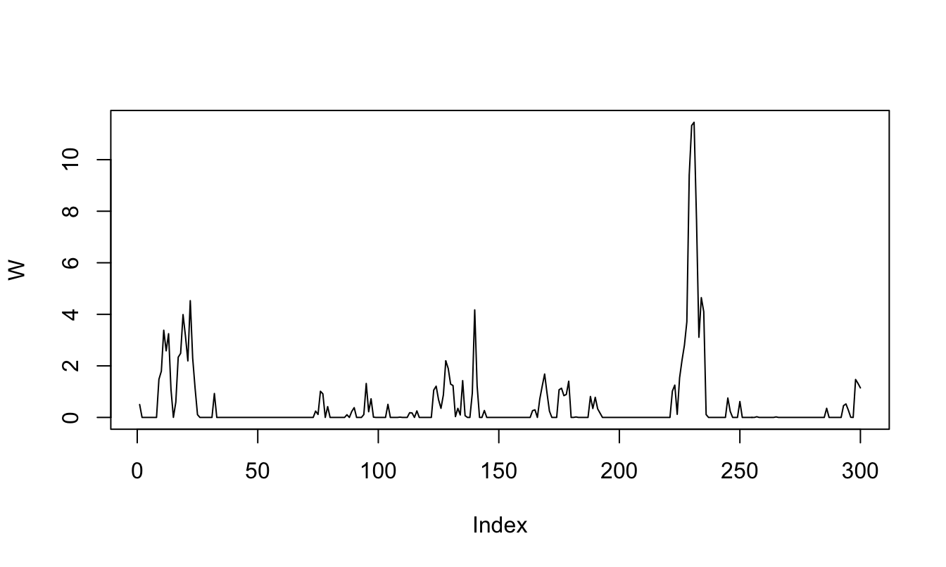

Figure 1.2: Simulation of an ARG0 processes.

Certain affine processes are valued in specific sets (e.g., integers). It is the case of compound Poisson proceses:

Example 1.9 (Compound Poisson process) A compound Poisson process is defined as follows (with $\gamma > 0$, $0 < \pi< 1$, and $\lambda > 0$): $$\frac{w_{t+1}}{\gamma} = z_{t+1} + \varepsilon_{t+1},$$ where $z_{t+1}$ and $\varepsilon_{t+1}$ conditionally independent, and where $z_{t+1} \sim {\mathcal B} \left(\frac{w_t}{\gamma},\pi\right)$, with $\varepsilon_{t+1} \sim {\mathcal P}(\lambda)$.

This process is valued in $\{j \gamma, j \in \mathbb{N}, \gamma \in \mathbb{R}^+\}$ and we have: $$\varphi_t(u) = \exp\left( \begin{array}{l} \dfrac{w_t}{\gamma} \log[\pi \exp(u\gamma)+1-\pi]-\lambda[1-\exp(u \gamma)] \end{array} \right),$$ i.e., $\varphi_t(u) = \exp\left(a(u)w_t+b(u)\right)$ with $$\left\{ \begin{array}{ccl} a(u)&=& \frac{1}{\gamma} \log[\pi \exp(u \gamma)+1-\pi],\\ b(u) &=& -\lambda[1-\exp(u \gamma)]. \end{array} \right.$$

We also have: $w_{t+1} = \pi w_t + \lambda \gamma + \eta_{t+1}$, where $\eta_{t+1}$ is a martingale difference.

One can simulate such processes by using this web-interface (select the “Compound Poisson” panel). Figure 1.3 makes use of function simul.compound.poisson (in package TSModels) to simulate a compound Poisson process.

library(TSModels)
W <- simul.compound.poisson(100,Gamma=.5,Pi=0.5,lambda=.9)
plot(W,type="l")

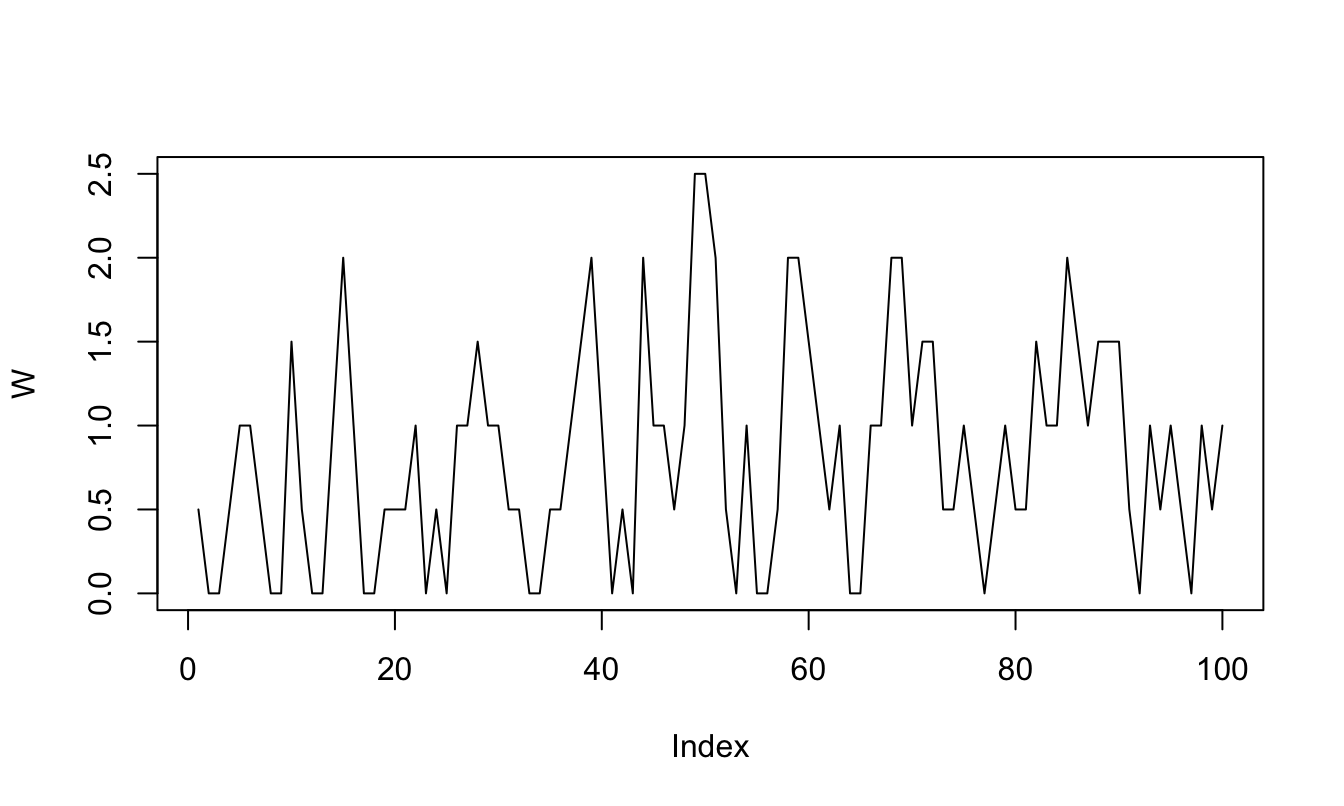
Figure 1.3: Simulation of a Compound Poisson process.

1.5.2 Affine processes of order $p$

Let us now define affine processes of order $p$:

Definition 1.2 (Affine process of order p) A multivariate process $w_{t+1}$ is affine of order $p$ if there exist functions $a_1(.),\dots,a_p(.)$, and $b(.)$ such that: $$\varphi_t(u)=\mathbb{E}_t[\exp(u' w_{t+1})]=\exp[a_1(u)'w_t+\dots+a_p(u)'w_{t+1-p}+b(u)].$$

It can be seen that if $w_t$ is affine of order $p$, then $W_t = [w_t', w_{t-1}',\dots,w_{t-p+1}']'$ is affine of order $1$.² Therefore, without loss of generality we can assume $p = 1$.

The standard affine processes of order $p$ are auto-regressive processes of order $p$. These processes satisfy the definition of index affine processes:

Definition 1.3 (Univariate index affine process of order p) Let $\exp[a(u)w_t+b(u)]$ be the conditional Laplace transform of a univariate affine process of order 1, the process $w_{t+1}$ is an index-affine process of order $p$ if: $$\varphi_t(u)=\mathbb{E}_t[\exp(u w_{t+1})]=\exp[a(u)(\beta_1 w_t+\dots+\beta_p w_{t+1-p})+b(u)].$$

Examples 1.10 and 1.11 are two examples of index affine processes.

Example 1.10 (Gaussian AR(p) process) This example extends Example 1.5. Consider a Gaussian AR(p) process $w_t$; that is: $$w_{t+1} = \nu + \varphi_1 w_t +\dots+ \varphi_p w_{t+1-p}+\sigma \varepsilon_{t+1},\quad \varepsilon_{t+1} \sim i.i.d. \mathcal{N}(0,1).$$ We have: $$\varphi_t(u) = \exp \left[ u \rho (\beta_1 w_t+\dots+\beta_p w_{t+1-p})+u\nu + u^2 \frac{\sigma^2}{2}\right]$$ with $\varphi_i = \rho \beta_i$.

Example 1.11 (ARG(p) process (positive)) This example extends Example 1.8. An ARG process of order $p$ is defined as follows: $$\frac{w_{t+1}}{\mu} \sim \gamma(\nu+z_t) \quad \mbox{where} \quad z_t \sim \mathcal{P} \left( \beta_1 w_t+\dots+\beta_p w_{t+1-p} \right),$$ with $\nu$, $\mu$, $\beta_i > 0$. We have: $$\varphi_t(u) = \exp\left[\frac{\rho u}{1-u \mu} (\beta_1 w_t+\dots+\beta_p w_{t+1-p})-\nu \log(1-u\mu)\right],$$ Process $w_t$ admits the following AR($p$) representation: $$w_{t+1} = \nu\mu + \varphi_1 w_t +\dots+ \varphi_p w_{t+1-p}+\varepsilon_{t+1},$$ with $\varphi_i = \beta_i\mu$ and where $\varepsilon_{t+1}$ is a martingale difference.

1.6 Markov chains

In this subsection, we show that the family of affine processes includes (some) regime-switching models. We consider a time-homogeneous Markov chain $z_t$, valued in the set of columns of $Id_J$, the identity matrix of dimension $J \times J$. The transition probabilities are denoted by $\pi(e_i, e_j)$, with $\pi(e_i, e_j) = \mathbb{P}(z_{t+1}=e_j | z_t=e_i)$. With these notations: $$\mathbb{E}[\exp(v'z_{t+1})|z_t=e_i,\underline{z_{t-1}}] = \sum^J_{j=1} \exp(v'e_j)\pi (e_i, e_j).$$ Hence, we have: $$\varphi_t(v) = \exp[a_z(v)'z_t],$$ with $$a_z(v)= \left[ \begin{array}{c} \log \left(\sum^J_{j=1} \exp(v'e_j) \pi(e_1,e_j)\right)\\ \vdots\\ \log \left(\sum^J_{j=1} \exp(v'e_j) \pi(e_J,e_j)\right) \end{array}\right].$$ This proves that $z_t$ is an affine process.

One can simulate a two-regime Markov chain by using this web-interface (select the “Markov-Switching” panel).

1.7 Wishart autoregressive (WAR) processes

WAR are matrix processes, valued in the space of $(L \times L)$ symmetric positive definite matrices.

Definition 1.4 (Wishart autoregressive (WAR) processes) Let $W_{t+1}$ be a $WAR_L(K, M, \Omega)$ process. It is defined by: $$\begin{eqnarray} &&\mathbb{E}[\exp Tr(\Gamma W_{t+1})|\underline{W_t}] \tag{1.5}\\ &=& \exp\left\{Tr[M'\Gamma(Id-2\Omega \Gamma)^{-1}M W_t] - \frac{K}{2} \log [det(Id-2\Omega \Gamma)]\right\}, \nonumber \end{eqnarray}$$ where $\Gamma$ is a symmetric matrix,³ $K$ is a positive scalar, $M$ is a $(L \times L)$ matrix, and $\Omega$ is a $(L \times L)$ symmetric positive definite matrix.

If $K$ is an integer, Proposition 1.4 (in the appendix) shows that $W_{t+1}$ can be simulated as: $$\begin{eqnarray*} \left\{ \begin{array}{ccl} W_{t+1} & =& \sum^K_{k=1} x_{k,t+1} x'_{k,t+1}\\ x_{k,t+1} &=& M x_{k,t} + \varepsilon_{k,t+1},\quad k \in \{1,\dots,K\}, \end{array} \right. \end{eqnarray*}$$ where $\varepsilon_{k,t+1} \sim i.i.d. \mathcal{N}(0, \Omega)$ (independent across $k$’s). The proposition also shows that we have: $$\mathbb{E}(W_{t+1}|\underline{W_t}) = MW_tM'+K \Omega,$$ i.e. $W_t$ follows a matrix weak AR(1) process.

In particular, when $L=1$ (univariate case), we have that: $$\begin{eqnarray*} \mathbb{E}[\exp(u W_{t+1})|\underline{W_t}] = \exp\left[ \frac{u m^2}{1-2\omega u}W_t - \frac{K}{2} \log(1-2\omega u)\right]. \end{eqnarray*}$$ Hence, when $L=1$, the Wishart process boils down to an $ARG(1)$ process (Example 1.8) with $\rho = m^2$, $\mu = 2\omega$, $\nu = \frac{K}{2}$.

1.8 Building affine processes

1.8.1 Univariate affine processes with stochastic parameters

Some univariate affine processes can be extended if they satisfy certain conditions. Specifically, consider a univariate affine process whose conditional L.T. is of the form: $$\begin{equation} \mathbb{E}_t \exp(u y_{t+1}) = \exp[a_0(u)y_t+b_0(u)'\delta],\tag{1.6} \end{equation}$$ where $\delta = (\delta_1,\dots,\delta_m)' \in \mathcal{D}$. This process can be generalized by making $\delta$ stochastic (while staying in the affine family). More precisely assume that: $$\mathbb{E}[\exp(u y_{t+1})|\underline{y_t}, \underline{z_{t+1}}] = \exp[a_0(u)y_t+b_0(u)'\Lambda z_{t+1}],$$ where $\Lambda$ is a $(m\times k)$ matrix, with $\Lambda z_{t+1} \in \mathcal{D}$. In this case, if: $$\mathbb{E}[\exp(v' z_{t+1})|\underline{y_t}, \underline{z_{t}}] = \exp[a_1(v)'z_t+b_1(v)],$$ then $w_{t+1} = (y_{t+1}, z'_{t+1})'$ is affine.⁴

Example 1.12 (Gaussian AR(p)) Using the notation of Example 1.10, it comes that an AR(p) processes satisfies (1.6) with $b_0(u) = \left(u, \; \frac{u^2}{2}\right)'$ and $\delta = (\nu,\sigma^2)' \in \mathcal{D}=\mathbb{R} \times \mathbb{R}^+$. In that case, $\delta$ (the vector of conditional mean and variance) can be replaced by …

• $\left( \begin{array}{l} z_{1,t+1} \\ z_{2,t+1} \end{array} \right)$, where $z_{1,t+1}$ and $z_{2,t+1}$ are independent AR(1) (see Example 1.5) and ARG(1) (see Example 1.8) processes, respectively.
• $\left( \begin{array}{ll} \lambda'_1 & 0 \\ 0 & \lambda'_2 \end{array} \right)$$\left( \begin{array}{l} z_{1,t+1} \\ z_{2,t+1} \end{array} \right)$, where $z_{1,t+1}$ and $z_{2,t+1}$ are independent Markov chains.
• $\left( \begin{array}{l} \lambda'_1 \\ \lambda'_2 \end{array}\right)z_{t+1}$, where $z_{t+1}$ is a Markov chain.

Example 1.11 (ARG(p) model) Consider Example 1.11, it comes that an ARG(p) processes satisfies (1.6), with $b_0(u) = - \nu \log(1-u\mu)$ and $\delta=\nu$. In that case, $\nu$ ($\ge 0$) can be specified for instance as a Markov chain or an ARG.

1.8.2 Multivariate affine processes

One can construct multivariate affine processes by employing the so-called recursive approach. Let us illustrate this by considering the bivariate case. (The multivariate generalization is straightforward.) Consider $w_t = \left(\begin{array}{c} w_{1,t}\\ w_{2,t} \end{array} \right)$, and assume that we have: $$\begin{eqnarray*} &&\mathbb{E}[\exp(u_1 w_{1,t+1}|\underline{w_{1,t}}, \underline{w_{2,t}})]\\ &=& \exp[a_{11}(u_1)w_{1,{\color{red}{t}}}+a_{12}(u_1)w_{2,{\color{red}{t}}}+b_{1}(u_1)], \end{eqnarray*}$$ (which defines $w_{1,t+1}|\underline{w_{1,t}}, \underline{w_{2,t}}$) and: $$\begin{eqnarray*} && \mathbb{E}[\exp(u_2 w_{2,t+1}|\underline{w_{1,t+1}}, \underline{w_{2,t}})]\\ &= & \exp[a_0(u_2)w_{1,{\color{red}{t+1}}}+a_{21}(u_2)w_{1,{\color{red}{t}}}+a_{22}(u_2)w_{2,{\color{red}{t}}}+b_2(u_2)] \end{eqnarray*}$$ (which defines $w_{2,t+1}|\underline{w_{1,t+1}}, \underline{w_{2,t}}$). Then $w_t$ is an affine process.⁵ The joint dynamics of the two components of $w_t$ can be expressed as: $$\begin{eqnarray*} w_{1,t+1} &=& \alpha_1 + \color{blue}{\alpha_{11}w_{1,t} + \alpha_{12}w_{2,t}} + \varepsilon_{1,t+1} \\ w_{2,t+1} &=& \alpha_2 + \alpha_{0}w_{1,t+1} + \color{blue}{\alpha_{21}w_{1,t} + \alpha _{22} w_{2,t}} + \varepsilon_{2,t+1}. \end{eqnarray*}$$ Note that $\varepsilon_{1,t+1}$ and $\varepsilon_{2,t+1}$ are non-correlated martingale differences. In the general case, they are conditionally heteroskedastic. What precedes is at play in $VAR$ model; Alain Monfort et al. (2017) employ this approach to build vector auto-regressive gamma (VARG) processes.

1.8.3 Extending multivariate stochastic processes

Consider the same framework as in Section 1.8.1 when $y_t$ is a $n$-dimensional vector. That is, replace (1.6) with: $$\begin{equation} \mathbb{E}_t \exp(u' y_{t+1}) = \exp[a_0(u)'y_t+b_0(u)\delta],\tag{1.7} \end{equation}$$ and further assume that $\delta$ is stochastic and depends on $z_t$, such that: $$\mathbb{E}[\exp(u y_{t+1})|\underline{y_t}, \underline{z_{t+1}}] = \exp[a_0'(u)y_t+b_0(u)\Lambda z_{t+1}],$$ where $\Lambda$ is a $(m\times k)$ matrix, with $\Lambda z_{t+1} \in \mathcal{D}$. In this case, if: $$\mathbb{E}[\exp(v' z_{t+1})|\underline{y_t}, \underline{z_{t}}] = \exp[a_1(v)'z_t+b_1(v)],$$ then $w_{t+1} = (y_{t+1}, z'_{t+1})'$ is affine.

Example 1.13 (Stochastic parameters Gaussian VAR(1)) This example extends Example 1.6. Using the same notations as in the latter example 1.6, we have $$b_0(u) = \left(u', \frac{1}{2} (u \otimes u)'\right)' \quad \mbox{and} \quad\delta = (\mu', vec(\Sigma)')' \in \mathbb{R}^n \times vec(\mathcal{S}),$$ where $\mathcal{S}$ is the set of symmetric positive semi-definite matrices. Vector $\delta$ can be replaced by $\left[ \begin{array}{l} z_{1,t+1} \\ z_{2,t+1}\end{array} \right]$, where

• $z_{1,t+1}$ is, for instance, a Gaussian VAR process.
• $z_{2,t+1}$ is
  • obtained by applying the $vec$ operator to a Wishart process,
  • replaced by $\Lambda_2 z_{2,t+1}$, where $\Lambda_2$ is a $(n^2 \times J)$ matrix whose columns are $vec(\Sigma_j)$, $j \in \{1,\dots,J\}$, the $\Sigma_j$ being $(n \times n)$ positive semi-definite, and $z_{2,t+1}$ is a selection vector of dimension $J \times 1$ or a standardized $J$-dimensional VARG process (multivariate extension of Example 1.8).

Example 1.14 (Regime-switching VAR(1)) One can also use this approach to construct (affine) regime-switching VAR processes (which is another extension of Example 1.6 (see, e.g., Christian Gourieroux et al. (2014)). For that, replace $\delta$ with

• $\left( \begin{array}{ll} \Lambda_1 & 0 \\ 0 & \Lambda_2 \end{array} \right)$$\left( \begin{array}{l} z_{1,t+1} \\ z_{2,t+1} \end{array} \right)$, where $\Lambda_1$ is a $(n \times J_1)$ matrix and $z_{1,t+1}$ is a Markov chain valued in the set of selection vectors of size $J_1$ (see Subsection 1.6), $\Lambda_2$ is the same matrix as in Example 1.13 and $z_{2,t+1}$ is a Markov chain valued in the set of selection vectors of size $J_2$.
• or $\left( \begin{array}{l} \Lambda_1 \\ \Lambda_2 \end{array}\right)z_{t+1}$, where $\Lambda_1$ and$\Lambda_2$ are the same matrices as above with $J_1=J_2=J$, and $z_{t+1}$ is a Markov chain valued in the set of selection vectors of size $J$.

1.8.4 Extended affine processes

Some processes are not affine, but may be sub-components of an affine process. This can be useful to compute their conditional moments and multi-horizon Laplace transform (as one can use the formulas presented above for that, using the enlarged—affine—vector).

Let us formally define an extended affine process:

Definition 1.5 (Extended Affine Processes) A process $w_{1,t}$ is extended affine if there exists a process $w_{2,t} = g(\underline{w_{1,t}})$ such that $(w'_{1,t}, w'_{2,t})'$ is affine (of order 1).

For an extended affine processes, $\varphi_{1,t}(u) = \mathbb{E}[\exp(u'w_{1,t+1})|\underline{w_{1,t}}]$ can be obtained from: $$\begin{eqnarray*} \varphi_t(u_1, u_2) &=& \mathbb{E}[\exp(u'_1w_{1,t+1}+u'_2 w_{2,t+1)}|\underline{w_{1,t}}, \underline{w_{2,t}}] \\ &=& \exp[a'_1(u_1,u_2)w_{1,t} + a'_2(u_1,u_2)w_{2,t}+b(u_1,u_2)] \end{eqnarray*}$$ by: $$\varphi_{1,t}(u) = \varphi_t(u, 0) = \exp[a'_1(u,0)w_{1,t}+a'_2(u,0)g(\underline{w_{1,t}}) + b(u, 0)].$$ In particular $w_{1,t}$ may be non-Markovian.

Similarly the multi-horizon Laplace transform (see Section 1.9) $$\mathbb{E}[\exp(\gamma'_{1}w_{1,t+1}+\dots+\gamma'_{h}w_{1,t+h})|\underline{w_{1,t}}]$$ can be obtained from the knowledge of the extended multi-horizon Laplace transform: $$\begin{eqnarray*} &&\mathbb{E}_t[\exp(\{\gamma'_{1,1}w_{1,t+1}+\gamma'_{2,1}w_{2,t+1}\}+\dots+ \{\gamma'_{1,h}w_{1,t+h}+\gamma'_{2,h}w_{2,t+h}\}] \\ &=& \exp[A'_{1,t,h}(\gamma^h_1, \gamma^h_2)w_{1,t}+A'_{2,t,h}(\gamma^h_1, \gamma^h_2)w_{2,t}+B_{t,h}(\gamma^h_1, \gamma^h_2)], \end{eqnarray*}$$ (with $\gamma^h_1 = (\gamma'_{1,1},\dots, \gamma'_{1,h})'$, and $\gamma^h_2 = (\gamma'_{2,1},\dots, \gamma'_{2,h})'$). We indeed have: $$\begin{eqnarray*} && \mathbb{E}[\exp(\gamma'_{1}w_{1,t+1}+\dots+\gamma'_{h}w_{1,t+h})|\underline{w_{1,t}}]\\ &=& \exp[A'_{1,t,h}(\gamma^h,0) w_{1,t} + A'_{2,t,h}(\gamma^h,0)g (\underline{w_{1,t}}) + B_{t,h}(\gamma^h,0)], \end{eqnarray*}$$ with $\gamma^h = (\gamma_1',\dots,\gamma_h')'$.

Example 1.15 (Affine process of order p) If $\{w_{1,t}\}$ is affine or order $p>1$, then $(w_{1,t},\dots,w_{1,t-p+1})$ is affine of order 1, but $\{w_{1,t}\}$ is not affine. That is, in that case, $w_{2,t} = (w'_{1,t-1}, \dots.w'_{1,t-p+1})'$.

This a kind of extreme case since $w_{2,t}$ belongs to the information at $t-1$, which implies $a_2(u_1, u_2) = u_2$.

Example 1.16 (Gaussian ARMA process) Consider an $ARMA(1,1)$ process $$w_{1,t} - \varphi w_{1,t-1} = \varepsilon_t-\theta \varepsilon_{t-1},$$ with $|\varphi | < 1$, $|\theta| < 1$, and $\varepsilon_t \sim i.i.d. \mathcal{N}(0, \sigma^2)$.

$w_{1,t}$ is not Markovian. Now, take $w_{2,t} = \varepsilon_t = (1-\theta L)^{-1}(1-\varphi L)w_{1,t}$. We have: $$\left( \begin{array}{l} w_{1,t+1} \\ w_{2,t+1} \end{array} \right) = \left( \begin{array}{ll} \varphi & -\theta \\ 0 & 0 \end{array} \right) \left( \begin{array}{l} w_{1,t} \\ w_{2,t} \end{array} \right) + \left( \begin{array}{l} 1 \\ 1 \end{array} \right) \varepsilon_{t+1}.$$ Hence $(w_{1,t}, w_{2,t})'$ follows a Gaussian $VAR(1)$, and, therefore, it is affine of order 1.

This is easily extended to $ARMA(p,q)$ and $VARMA(p,q)$ processes.

Example 1.17 (GARCH type process) Consider process $w_{1,t}$, defined by: $$w_{1,t+1} = \mu + \varphi w_{1,t} + \sigma_{t+1} \varepsilon_{t+1},$$ where $|\varphi| < 1$ and $\varepsilon_t \sim i.i.d. \mathcal{N}(0,1)$, and $$\sigma^2_{t+1} = \omega + \alpha \varepsilon^2_t + \beta \sigma^2_t,$$ where $0 < \beta < 1$.

Consider $w_{2,t} = \sigma^2_{t+1}$ (which is a non-linear function of $\underline{w_{1,t}}$). Proposition 1.7 shows that: $$\begin{eqnarray*} && \mathbb{E}\left[\exp(u_1 w_{1,t+1} + u_2 w_{2,t+1})|\underline{w_{1,t}}\right] \\ &=& \exp\left[u_1 \mu + u_2 \omega - \frac{1}{2} \log(1-2 u_2 \alpha) \right. \\ &&\left. + u_1 \varphi w_{1,t} + (u_2\beta + \frac{u^2_1}{2(1-2u_2\alpha)}) w_{2,t}\right], \end{eqnarray*}$$ which is exponential affine in $(w_{1,t}, w_{2,t})$.

1.9 Multi-horizon Laplace transform

1.9.1 Recursive computation and direct pricing implications

In this subsection, we show that multi-horizon Laplace transforms of affine processes can be calculated recursively. Various examples will show how this can be exploited to price long-dated financial instruments.

Let us consider a multivariate process $w_{t}$, affine of order one. (As explained in Subsection 1.5.2, this includes the case of the order $p$ case.) For the sake of generality, we consider the case where functions $a(.)$, $b(.)$ are possibly deterministic functions of time, denoted in this case $a_{t+1}(.)$ and $b_{t+1}(.)$: $$\mathbb{E}_t \exp[(u'w_{t+1})] = \exp[a'_{t+1}(u)w_t+b_{t+1}(u)].$$ The multi-horizon Laplace transform associated with date $t$ and horizon $h$ is defined by: $$\begin{equation} \varphi_{t,h}(\gamma_1,\dots,\gamma_h) = \mathbb{E}_t[\exp(\gamma'_1w_{t+1}+\dots+\gamma'_h w_{t+h})].\tag{1.8} \end{equation}$$

Lemma 1.5 (in the appendix) shows that we have: $$\varphi_{t,h}(\gamma_1,\dots,\gamma_h) = \exp(A'_{t,h} w_t + B_{t,h}),$$ where $A_{t,h} = A^h_{t,h}$ and $B_{t,h} = B^h_{t,h}$, the $A^h_{t,i}, B^h_{t,i}$ $i = 1,\dots,h$, being given recursively by: $$\left\{ \begin{array}{ccl} A^h_{t,i} &=& a_{t+h+1-i}(\gamma_{h+1-i} + A^h_{t,i-1}), \\ B^h_{t,i} &=& b_{t+h+1-i}(\gamma_{h+1-i} + A^h_{t,i-1}) + B^h_{t,i-1}, \\ A^h_{t,0} &=& 0, B^h_{t,0} = 0. \end{array} \right.$$

If the functions $a_{t}$ and $b_{t}$ do not depend on $t$, these recursive formulas do not depend on $t$, and we get $\varphi_{t,h}(\gamma_1,\dots,\gamma_h)$, for any $t$, with only one recursion for each $h$.

Moreover, if the functions $a_{t}$ and $b_{t}$ do not depend on $t$, and if different sequences $(\gamma^h_1,\dots,\gamma^h_h), h=1,\dots,H$ (say) satisfy $\gamma^h_{h+1-i} = u_i$, for $i=1,\dots,h$, and for any $h \leq H$, that is if we want to compute (reverse-order case): $$\begin{equation} \varphi_{t,h}(u_h,\dots,u_1)=\mathbb{E}_t[\exp(u'_{{\color{red}h}} w_{{\color{red}t+1}}+\dots+u'_{{\color{red}1}} w_{{\color{red}t+h}})], \quad h=1,\dots,H,\tag{1.9} \end{equation}$$ then Proposition 1.5 (in the appendix) shows that we can compute the $\varphi_{t,h}(u_h,\dots,u_1)$ for any $t$ and any $h \leq H$ with only one recursion. That is $\varphi_{t,h}(u_h,\dots,u_1)=\exp(A'_hw_t+B_h)$ with: $$\begin{equation*} \left\{ \begin{array}{ccl} A_{h} &=& a(u_{h} + A_{h-1}), \\ B_{h} &=& b(u_{h} + A_{h-1}) + B_{h-1}, \\ A_{0} &=& 0,\quad B_{0} = 0. \end{array} \right. \end{equation*}$$

As mentioned above, what precedes has useful implications to price long-dated financial instruments such as nominal and real bonds (Examples 1.18 and 1.20, respectively), or futures (Example 1.21).

Example 1.18 (Nominal interest rates) Let $B_{t,h}$ denote the date-$t$ price of a nominal zero-coupon bond of maturity $h$. We have (see (2.3) and Subsection 4.2.1): $$\begin{equation} B_{t,h} = \mathbb{E}^{\mathbb{Q}}_t \exp (-i_{t}-\dots-i_{t+h-1}),\tag{1.10} \end{equation}$$ where $i_{t}$ is the nominal short rate between $t$ and $t+1$ (observed at $t$), and the associated (continuously-compounded) yield-to-maturity is given by: $$\begin{equation} i_{t,h} = - \frac{1}{h} \log B(t,h), \quad h=1,\dots,H. \end{equation}$$ If $i_t = \omega'w_t$ (say), then: $$B_{t,h} = \exp(-i_{t}) \mathbb{E}^{\mathbb{Q}}_t \exp(-\omega' w_{t+1} - \dots - \omega' w_{t+h-1}).$$ One can then price this bond by directly employing (1.9), with $u_1 = 0$ and $u_i = - \omega$, $i = 2,\dots, H$. The price $B_{t,h}$ is exponential affine in $w_t$, the associated yield-to-maturity $i_{t,h}=-1/h\log B_{t,h}$ is affine in $w_t$.

Example 1.19 (No-arbitrage Nelson-Siegel model) In this example, we employ the results of Example 1.18 in the context described by Christensen, Diebold, and Rudebusch (2009). Specifically, we consider a three factor model following a Gaussian VAR (see Example 1.6): $$w_t = \left[\begin{array}{c}X_{1,t}\\X_{2,t}\\X_{3,t}\end{array}\right] = \left[\begin{array}{ccc} 1 & 0 & 0\\ 0&1-\lambda&\lambda\\ 0&0&1-\lambda\end{array}\right] \left[\begin{array}{c}X_{1,t-1}\\X_{2,t-1}\\X_{2,t-1}\end{array}\right] + \left[\begin{array}{ccc} \sigma_{11} & 0 & 0\\ \sigma_{21}&\sigma_{22}&0\\ \sigma_{31}&\sigma_{32}&\sigma_{33}\end{array}\right] \left[\begin{array}{c}\varepsilon_{1,t}\\\varepsilon_{2,t}\\\varepsilon_{3,t}\end{array}\right],$$ where $\left[\begin{array}{c}\varepsilon_{1,t}\\\varepsilon_{2,t}\\\varepsilon_{3,t}\end{array}\right] \sim \,i.i.d.\, \mathcal{N}(0,Id)$.

The nominal short-term rate is given by $i_t = X_{1,t}+X_{2,t}$. In that case, we can use the results of Example 1.18 with $\omega = (-1,-1,0)'$. The following lines of code do that:

library(TSModels)
lambda <- .05
Phi <- diag(c(1,1-lambda,1-lambda));Phi[2,3] <- lambda
Sigma <- .0005 * diag(3)
psi.parameterization=list(mu=matrix(0,3,1),Phi=Phi,Sigma=Sigma)
u1 <- matrix(0,3,1)
u2 <- matrix(c(-1,-1,0),ncol=1)
H <- 20
AB <- reverse.MHLT(psi.GaussianVAR,u1 = u1,u2 = u2,H = H,
                   psi.parameterization = psi.parameterization)
AB$A[1:2,,] <- AB$A[1:2,,] - 1 # add terms for exp(-i_t)
a.yield <- - AB$A / array((1:H) %x% rep(1,3),c(3,1,H))
b.yield <- - AB$B / array((1:H) %x% rep(1,3),c(1,1,H))
plot(a.yield[1,,],type="l",lwd=2,ylim=c(0,1),
     xlab="Maturity",ylab="Factor loadings")
lines(a.yield[2,,],col="red",lwd=2,lty=2)
lines(a.yield[3,,],col="blue",lwd=2,lty=3)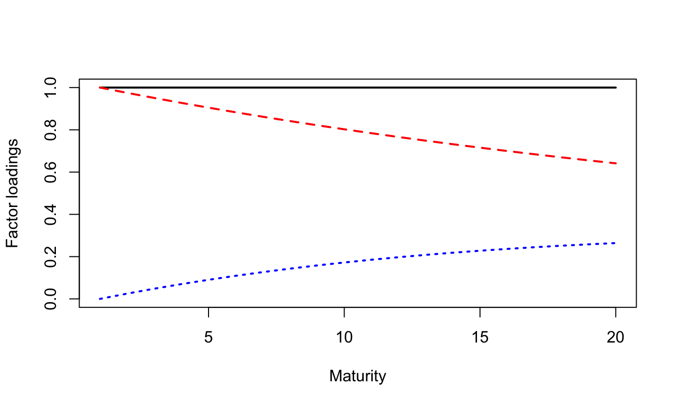

Figure 1.4: Factor loadings in the context of a no-arbitrage nelson-Siegel model (Christensen, Diebold and Rudebusch, 2009). The first factor (black solid line) is a level factor. The second and third factors (red dashed line and blue dotted line, respectively) are slope factors.

Christensen, Diebold, and Rudebusch (2009) show that such specifications allow to approximate the widely-used C. R. Nelson and Siegel (1987) yield curve specification.⁶

In the previous example, note the use of function reverse.MHLT (in package TSModels), that notably takes a L.T. as an argument (psi). In the previous example, we consider a Gaussian VAR, and we therefore assign psi.GaussianVAR to psi. We then need to provide function reverse.MHLT with the arguments of the psi function. These arguments are provided in the form of a list (input psi.parameterization).

Example 1.20 (Real interest rates) Denote by $q_t$ the price index on date $t$ and by $\pi_{t+1} = \log \dfrac{q_{t+1}}{q_t}$ the log-inflation rate between dates $t$ and $t+1$. The real rate of maturity $h$ is given by (see Subsection 4.2.1): $$\begin{eqnarray*} r_{t,h} & =& - \frac{1}{h} \log \mathcal{B}_{t,h}, \quad h=1,\dots,H \\ \\ \mathcal{B}_{t,h} & =& \mathbb{E}^{\mathbb{Q}}_t \exp(-i_{t}-\dots-i_{t+h-1} + \pi_{t+1}+\dots+\pi_{t+h}), \\ \\ & =& \exp(-i_{t}) \times \\ && \mathbb{E}^{\mathbb{Q}}_t \exp(-i_{t+1}-\dots-i_{t+h-1}+\pi_{t+1}+\dots+\pi_{t+h}), \end{eqnarray*}$$ where $i_t$ is the nominal short-term rate and $\mathcal{B}_{t,h}$ is the price of a real zero-coupon bond of maturity $h$ (which is also a inflation-indexed zero-coupon bond). If $i_t = \omega'w_t$ and $\pi_t = \bar\omega'w_t$, then $\mathcal{B}_{t,h}$ is given by: $$\begin{eqnarray*} \exp(-i_{t}) \mathbb{E}^{\mathbb{Q}}_t \exp[(\bar\omega-\omega)'w_{t+1}+\dots+(\bar\omega-\omega)'w_{t+h-1}+\bar\omega' w_{t+h}]. \end{eqnarray*}$$ One can then price this bond by directly employing (1.9), with $u_1 = \bar\omega$ and $u_i = \bar\omega-\omega$, $i = 2,\dots, H$.

Example 1.21 (Futures) Denote by $F(t,h)$ the date-$t$ price of a future of maturity $h$ (see Subsection 6.1.2). That is $F(t,h) = \mathbb{E}^{\mathbb{Q}}_t (S_{t+h})$, $h=1,\dots,H$, where $S_t$ is the date-$t$ price of the underlying asset.

• If $w_t = (\log S_t, x'_t)'$ then $F(t,h) = \mathbb{E}^{\mathbb{Q}}_t \exp(e'_1 w_{t+h})$. This can be calculated by using (1.9) with $u_1 = e_1$, and $u_i = 0$, for $i=2,\dots,H$.

• If $w_t = (y_t, x'_t)'$ with $y_t = \log\frac{S_t}{S_{t-1}}$, then $F(t,h) = S_t \mathbb{E}^{\mathbb{Q}}_t \exp(e'_1 w_{t+1}+\dots+e'_1 w_{t+h})$. This can be calculated by using (1.9) with $u_i = e'_1$, $i=1,\dots,H$.

1.9.2 Exponential payoff

Consider an asset providing the payoff $\exp(\nu' w_{t+h})$ on date $t+h$. Its price is given by: $$P(t,h;\nu) = \mathbb{E}^{\mathbb{Q}}_t[\exp(-i_{t}-\dots-i_{t+h-1}) \exp(\nu' w_{t+h})].$$ If $i_t = \omega'w_t$, we have: $$P(t,h;\nu) = \exp(-r_{t})\mathbb{E}^{\mathbb{Q}}_t \left(\exp[-\omega' w_{t+1}-\dots-\omega' w_{t+h-1}+ \nu' w_{t+h}]\right),$$ which can be calculated by (1.9), with $u_1 = \nu$ and $u_i = -\omega$ for $i = 2,\dots,H$.

What precedes can be extended to the case where the payoff (settled on date $t+h$) is of the form: $$(\nu_1'w_{t+h}) \exp(\nu_2' w_{t+h}).$$ Indeed, we have $$\left[\frac{\partial \exp[(s \nu_1+ \nu_2)'w_{t+h}]}{\partial s}\right]_{s=0} = (\nu_1'w_{t+h}) \exp(\nu_2' w_{t+h}).$$ Therefore: $$\begin{eqnarray} &&\mathbb{E}_t^{\mathbb{Q}}[\exp(-i_t - \dots - i_{t+h-1})(\nu_1'w_{t+h}) \exp(\nu_2' w_{t+h})] \nonumber\\ &=& \left[ \frac{\partial P(t,h;s \nu_1 + \nu_2)}{\partial s} \right]_{s=0}.\tag{1.11} \end{eqnarray}$$ This method is easily extended to price payoffs of the form $(\nu_1'w_{t+h})^k \exp(\nu_2' w_{t+h})$, with $k \in \mathbb{N}$.

1.10 VAR representation and conditional moments

An important property of affine processes is that their dynamics can be written as a vector-autoregressive process. This is useful, in particular, to compute conditional moments of the process.

Proposition 1.1 (VAR representation of an affine process' dynamics) If $w_t$ is the affine process whose Laplace transform is defined in Def. 1.1, then its dynamics admits the following vectorial autoregressive representation: $$\begin{equation} w_{t+1} = \mu + \Phi w_{t} + \Sigma^{\frac{1}{2}}(w_t) \varepsilon_{t+1},\tag{1.12} \end{equation}$$ where $\varepsilon_{t+1}$ is a difference of martingale sequence whose conditional covariance matrix is the identity matrix and where $\mu$, $\Phi$ and $\Sigma(w_t) = \Sigma^{\frac{1}{2}}(w_t){\Sigma^{\frac{1}{2}}(w_t)}'$ satisfy: $$\begin{equation} \mu = \left[\frac{\partial }{\partial u}b(u)\right]_{u=0}, \quad \Phi= \left[\frac{\partial }{\partial u}a(u)'\right]_{u=0}\tag{1.13} \end{equation}$$ $$\begin{equation} \Sigma(w_t) = \left[\frac{\partial }{\partial u\partial u'}b(u)\right]_{u=0} + \left[\frac{\partial }{\partial u\partial u'}a(u)'w_t\right]_{u=0}.\tag{1.14} \end{equation}$$

Proof. When $w_t$ is affine, its (conditional) cumulant generating function is of the form $\psi(u)=a(u)'w_t+b(u)$. The result directly follows from the formulas given in Section 1.3.

Proposition 1.6 (in the appendix) further shows that the conditional multi-horizon means and variances of $w_t$ are given by: $$\begin{eqnarray} \mathbb{E}_t(w_{t+h}) &=& (I - \Phi)^{-1}(I - \Phi^h)\mu + \Phi^h w_t \tag{1.15}\\ \mathbb{V}ar_t(w_{t+h}) &=& \Sigma(\mathbb{E}_t(w_{t+h-1}))+\Phi \Sigma(\mathbb{E}_t(w_{t+h-2}))\Phi' + \nonumber \\ && \dots + \Phi^{h-1} \Sigma(w_{t}){\Phi^{h-1}}'. \tag{1.16} \end{eqnarray}$$ Eq. (1.16) notably implies that $\mathbb{V}ar_t(w_{t+h})$ is an affine function of $w_t$. Indeed $\Sigma(.)$ is an affine function, and the conditional expectations $\mathbb{E}_t(w_{t+h})$ are affine in $w_t$, as shown by (1.15).

The unconditional means and variances of $w_t$ are given by: $$\begin{equation} \left\{ \begin{array}{ccl} \mathbb{E}(w_t) &=& (I - \Phi)^{-1}\mu\\ vec[\mathbb{V}ar(w_t)] &=& (I_{n^2} - \Phi \otimes \Phi)^{-1} vec\left(\Sigma[(I - \Phi)^{-1}\mu]\right). \end{array} \right.\tag{1.17} \end{equation}$$

1.11 Truncated Laplace transforms of affine processes

In this section, we show how one can employ Fourier transforms to compute truncated conditional moments of affine processes. For that, let us introduce the following notation: $$w_{t+1,T} = (w'_{t+1}, w'_{t+2},\dots, w'_T)'$$ with $w_t$ affine $n$-dimensional process.

We want to compute: $$\tilde{\varphi}_t(u ; v, \gamma) = \mathbb{E}_t[\exp(u'w_{t+1,T})\textbf{1}_{\{v'w_{t+1,T}<\gamma\}}].$$

Consider the complex untruncated conditional Laplace transform: $$\varphi_t(z) = \mathbb{E}_t[\exp(z'w_{t+1,T})],\quad z \in \mathbb{C}^{nT},$$ computed using the same recursive algorithm as in the real case (see Section 1.9).

Darrell Duffie, Pan, and Singleton (2000) have shown that we have (see also Proposition 1.8 in the appendix): $$\begin{equation} \tilde{\varphi}_t(u ; v, \gamma) = \frac{\varphi_t(u)}{2} - \frac{1}{\pi} \int^\infty_0 \frac{Im[\varphi_t(u+ivx) \exp(-i\gamma x)]}{x} dx.\tag{1.18} \end{equation}$$ where $Im$ means imaginary part.

Note that the integral in (1.18) is one dimensional (whatever the dimension of $w_t$). As shown in the following example, this can be exploited to price options.

Example 1.22 (Option pricing) Pricing calls and puts amounts to conditional expectations of the type (with $k > 0$): $$\begin{eqnarray*} && \mathbb{E}_t\left([\exp(u'_1 w_{t+1,T})-k \exp(u'_2 w_{t+1,T})]^+\right) \\ &= & \mathbb{E}_t\left([\exp(u'_1 w_{t+1,T})-k \exp(u'_2 w_{t+1,T})]\textbf{1}_{\{[\exp(u_1-u_2)'w_{t+1,T}] > k \}}\right) \\ &= & \tilde{\varphi}_t(u_1 ; u_2-u_1, - \log k) - k \tilde{\varphi}_t(u_2 ; u_2-u_1, - \log k). \end{eqnarray*}$$

Example 1.23 (Exogenous short rate) Consider an asset whose date-$t$ price is $p_t$. Denote its geometric asset return by $y_t$, i.e., $y_t = \log(p_t/p_{t-1})$. Consider an option written on this asset, with a strike equal $k p_t$.

If interest rates are deterministic, the option price, for a maturity $h$, is given by: $$p_t \exp(-i_{t}-\dots-i_{t+h-1}) \mathbb{E}^{\mathbb{Q}}_t[\exp u'_1 w_{t+1, t+h} - k]^+$$ with $u_1 = e \otimes e_1$, where $e$ is the $h$-dimensional vector with components equal to 1, and $e_1$ is the $n$-vector selecting the 1st component ($y_t$ being the 1st component of $w_t$, say).

Example 1.24 (Endogenous short rate) Consider the same context as in Example 1.23, but with a stochastic (endogenous) short-term rate. For instance, assume that $i_{t+1} = \omega_0 + \omega'_1 w_t$. The option price then is: $$\begin{eqnarray*} && p_t \mathbb{E}^{\mathbb{Q}}_t \left[ \exp(-\omega_0 - \omega'_1 w_t-\dots- \omega_0 - \omega'_1 w_{t+h-1}) [\exp(u'_1 w_{t+1,t+h})-k]^+ \right]\\ &= & p_t \exp(-h \omega_0 - \omega'_1 w_t)\mathbb{E}^{\mathbb{Q}}_t\left(\left[\exp(\tilde{u}'_1w_{t+1,t+h})-k \exp(u_2 w_{t+1, t+h})\right]^+\right), \end{eqnarray*}$$ with $\tilde{u}'_1 = u_1 + u_2$, [$u_1 = e \otimes e_1$ as before], and $u_2 = (-\omega'_1,\dots, -\omega'_1, 0)'$.

Example 1.25 (Numerical example: Conditional cumulated distribution function (c.d.f.)) Let us use the model used in Example 1.19. Suppose we want to compute the conditional distribution of the average interest rate over the next $H$ periods, i.e., $\frac{1}{H}(i_{t+1}+\dots+i_{t+H})$. Hence, we want to compute $\mathbb{E}_t[\textbf{1}_{\{v'w_{t+1,T}<\gamma\}}]$ with $v'w_{t+1,T}=\frac{1}{H}(i_{t+1}+\dots+i_{t+H})$.

H  <- 10
X  <- matrix(c(0.01,.02,0),3,1)
x  <- exp(seq(-10,10,length.out=1000))
u1 <- matrix(c(1/H,1/H,0),3,1) %*% matrix(1i*x,nrow=1);u2 <- u1
AB <- reverse.MHLT(psi.GaussianVAR,u1 = u1,u2 = u2,H = H,
                   psi.parameterization = psi.parameterization)
s1 <- matrix(exp(t(X) %*% AB$A[,,H] + AB$B[,,H]),ncol=1)
dx <- matrix(x-c(0,x[1:length(x)-1]),length(x),1)
gamma <- seq(-.2,.3,length.out=1000)
fx <- outer(x,gamma,function(r,c){Im(s1[,1]*
                                       exp(-1i*r*c))/r})*dx[,1]
f  <- 1/2 - 1/pi * apply(fx,2,sum)
plot(gamma,f,type="l",xlab="",lwd=2)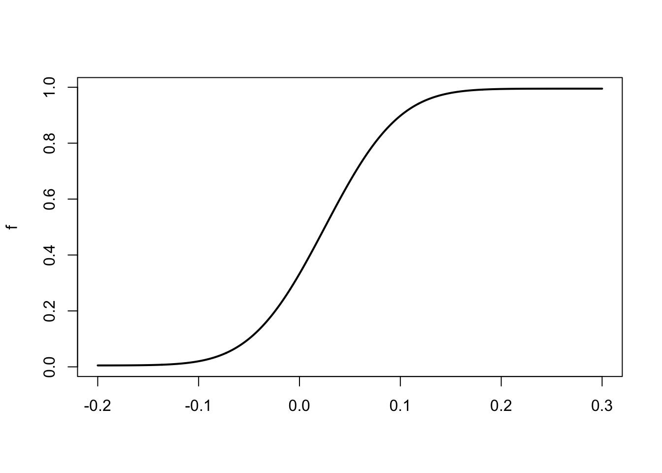

Figure 1.5: Conditional cumulated distribution function (c.d.f.) of $\frac{1}{H}(i_{t+1}+\dots+i_{t+H})$.

1.12 Appendices

Lemma 1.3 If $\mu \in \mathbb{R}^L$ and $Q$ is a $(L \times L)$ matrix symmetric positive definite, then: $$\int_{\mathbb{R}^{L}} \exp(-u'Q u + \mu'u)du = \frac{\pi^{L/2}}{(det Q)^{1/2}} \exp \left( \begin{array}{l} \frac{1}{4} \mu'Q^{-1}\mu \end{array} \right).$$

Proof. The integral is: $$\begin{eqnarray*} && \int_{\mathbb{R}^{L}} exp \left[ \begin{array}{l} - (u - \frac{1}{2} Q^{-1} \mu)' Q (u - \frac{1}{2} Q^{-1} \mu)' \end{array} \right] exp\left( \begin{array}{l} \frac{1}{4} \mu'Q^{-1}\mu \end{array} \right)du \\ &=& \frac{\pi^{L/2}}{(det Q)^{1/2}} exp\left( \begin{array}{l} \frac{1}{4} \mu'Q^{-1}\mu \end{array} \right) \end{eqnarray*}$$ [using the formula for the unit mass of $\mathcal{N}( 0.5Q^{-1}\mu,(2Q)^{-1})$].

Lemma 1.4 If $\varepsilon_{t+1} \sim \mathcal{N}(0,Id)$, we have $$\mathbb{E}_t \left(\exp[\lambda'\varepsilon_{t+1}+\varepsilon'_{t+1} V \varepsilon_{t+1}]\right) = \frac{1}{[\det(I-2V)]^{1/2}} \exp\left[ \frac{1}{2} \lambda'(I-2V)^{-1}\lambda \right].$$

Proof. We have $$\mathbb{E}_t \exp(\lambda'\varepsilon_{t+1}+\varepsilon'_{t+1}V\varepsilon_{t+1}) = \frac{1}{(2\pi)^{n/2}} \int_{\mathbb{R}^{n}} \exp\left[ \begin{array}{l} -u'\left( \begin{array}{l} \frac{1}{2} I-V \end{array} \right)u+\lambda'u \end{array} \right]du$$ From Lemma 1.3, if $u\in\mathbb{R}^n$, then $$\int_{\mathbb{R}^{n}} \exp(-u' Q u+\mu'u) du = \frac{\pi^{n/2}}{(\det Q)^{1/2}} \exp\left( \begin{array}{l} \frac{1}{4} \mu'Q^{-1}\mu \end{array} \right).$$ Therefore: $$\begin{array}{l} \mathbb{E}_t \exp(\lambda'\varepsilon_{t+1}+\varepsilon'_{t+1}V\varepsilon_{t+1}) \\ = \frac{1}{2^{n/2} \left[ \begin{array}{l} \det \left( \begin{array}{l} \frac{1}{2} I-V \end{array} \right) \end{array} \right]^{1/2} } \exp\left[ \begin{array}{l} \frac{1}{4} \lambda'\left( \begin{array}{l} \frac{1}{2} I-V \end{array} \right)^{-1}\lambda \end{array} \right]. \end{array}$$

Proposition 1.2 (Quadratic Gaussian process) Consider vector $w_t = (x'_t,vec(x_t x_t')')'$, where $x_t$ is a $n$-dimensional vector following a Gaussian VAR(1), i.e. $$x_{t+1}|\underline{w_t} \sim \mathcal{N}(\mu+\Phi x_t, \Sigma).$$ If $u = (v,V)$ where $v \in \mathbb{R}^n$ and $V$ a square symmetric matrix of size $n$, we have: $$\begin{eqnarray*} \varphi_t(u) &=& \mathbb{E}_t\big\{\exp\big[(v',vec(V)')\times w_{t+1}\big]\big\} \\ & =& \exp \left\{a_1(v,V)'x_t +vec(a_2(v,V))' vec(x_t'x_t) + b(v,V) \right\}, \end{eqnarray*}$$ where: $$\begin{eqnarray*} a_2(u) & = & \Phi'V (I_n - 2\Sigma V)^{-1} \Phi \nonumber \\ a_1(u) & = & \Phi'\left[(I_n-2V\Sigma)^{-1}(v+2V\mu)\right] \nonumber \\ b(u) & = & u'(I_n - 2 \Sigma V)^{-1}\left(\mu + \frac{1}{2} \Sigma v\right) +\\ && \mu'V(I_n - 2 \Sigma V)^{-1}\mu - \frac{1}{2}\log\big|I_n - 2\Sigma V\big|.\tag{1.3} \end{eqnarray*}$$

Proof. We have: $$\begin{eqnarray*} &&\mathbb{E}_t(\exp(v' x_{t+1} + vec(V)'vec(x_{t+1} x_{t+1}'))) \\ &=& \mathbb{E}_t[\exp(v' (\mu + \Phi x_t + \Sigma^{1/2}\varepsilon_{t+1}) + \\ && vec(V)'vec((\mu + \Phi x_t + \Sigma^{1/2}\varepsilon_{t+1}) (\mu + \Phi x_t + \Sigma^{1/2}\varepsilon_{t+1})'))] \\ &=& \exp[v' (\mu + \Phi x_t) + vec(V)'vec\{(\mu + \Phi x_t)(\mu + \Phi x_t)'\}] \times \\ && \mathbb{E}_t[\exp(v'\Sigma^{1/2}\varepsilon_{t+1} +2\underbrace{ vec(V)' vec\{(\mu + \Phi x_t)(\varepsilon_{t+1}'{\Sigma^{1/2}}')\}}_{=(\mu + \Phi x_t)'V\Sigma^{1/2}\varepsilon_{t+1}} +\\ && \underbrace{vec(V)'vec\{(\Sigma^{1/2}\varepsilon_{t+1})(\Sigma^{1/2}\varepsilon_{t+1})'}_{=\varepsilon_{t+1}'{\Sigma^{1/2}}'V\Sigma^{1/2}\varepsilon_{t+1}}\}]. \end{eqnarray*}$$ Lemma 1.4 can be used to compute the previous conditional expectation, with $\lambda = {\Sigma^{1/2}}'(v + 2 V'(\mu + \Phi x_t))$. Some algebra then leads to the result.

Proposition 1.3 () Consider the following auto-regressive gamma process: $$\frac{w_{t+1}}{\mu} \sim \gamma(\nu+z_t) \quad \mbox{where} \quad z_t \sim \mathcal{P} \left( \frac{\rho w_t}{\mu} \right),$$ with $\nu$, $\mu$, $\rho > 0$. (Alternatively $z_t \sim {\mathcal{P}}(\beta w_t)$, with $\rho = \beta \mu$.)

We have: $\varphi_t(u) = exp \left[ \begin{array}{l} \dfrac{\rho u}{1-u \mu} w_t - \nu \log(1-u \mu)\end{array} \right], \mbox{ for } u < \dfrac{1}{\mu}$.

Proof. Given $\underline{w_t}$, we have $z_t \sim {\mathcal P}\left( \begin{array}{l} \frac{\rho w_t} {\mu} \end{array}\right)$. We have: $$\begin{eqnarray*} \mathbb{E}[\exp(u w_{t+1})|\underline{w_t}] &=& \mathbb{E}\left\{\mathbb{E}\left[\exp \left(u \mu \frac{w_{t+1}}{\mu}\right)|\underline{w_t}, \underline{z}_t\right]\underline{w_t}\right\}\\ &=& \mathbb{E}[(1-u\mu)^{-(\nu+z_t)}|\underline{w_t}] \\ &=& (1-u\mu)^{-\nu}\mathbb{E}\{\exp[-z_t \log(1-u\mu)]|\underline{w_t}\} \\ &=& (1-u\mu)^{-\nu} \exp \left\{\frac{\rho w_t}{\mu}[\exp(-\log(1-u\mu)] - \frac{\rho w_t}{\mu}\right\}\\ &=& \exp\left[ \begin{array}{l} \frac{\rho u w_t}{1-u\mu} - \nu \log(1-u\mu) \end{array}\right], \end{eqnarray*}$$ using the fact that the L.T. of $\gamma(\nu)$ is $(1-u)^{-\nu}$ and that the L.T. of ${\mathcal P}(\lambda)$ is $\exp[\lambda(\exp(u)-1)]$.

Proposition 1.4 (Dynamics of a WAR process) If $K$ is an integer, $W_{t+1}$ can be obtained from: $$\begin{eqnarray*} \left\{ \begin{array}{ccl} W_{t+1} & =& \sum^K_{k=1} x_{k,t+1} x'_{k,t+1}\\ &&\\ x_{k,t+1} & =& M x_{k,t} + \varepsilon_{k,t+1},\quad k \in \{1,\dots,K\}, \end{array} \right. \end{eqnarray*}$$ where $\varepsilon_{k,t+1} \sim i.i.d. \mathcal{N}(0, \Omega)$ (independent across $k$’s). In particular, we have: $$\mathbb{E}(W_{t+1}|\underline{W_t}) = MW_tM'+K \Omega,$$ i.e. $W_t$ follows a matrix weak AR(1) process.

Proof. For $K=1$, $W_{t+1}=x_{t+1} x'_{t+1}$, $x_{t+1} = M x_t + \Omega^{1/2} u_{t+1}$ and $u_{t+1} \sim i.i.d. \mathcal{N}(0,Id_L)$. We have: $$\mathbb{E}[\exp(Tr \Gamma W_{t+1})|\underline{w_t}] = \mathbb{E}\{\mathbb{E}[\exp(Tr \Gamma x_{t+1} x'_{t+1})|\underline{x}_t]|\underline{w_t}\}$$ and: $$\begin{eqnarray*} && \mathbb{E}[\exp(Tr \Gamma x_{t+1}x'_{t+1})|\underline{x}_t] = \mathbb{E}[\exp(x'_{t+1}\Gamma x_{t+1}|\underline{x}_t] \\ &=& \mathbb{E}[\exp(M x_t + \Omega^{1/2} u_{t+1})'\Gamma(M x_t + \Omega^{1/2} u_{t+1})/x_t] \\ &=& \exp(x'_tM'\Gamma M x_t)\mathbb{E}[\exp(2 x'_t M'\Gamma \Omega^{1/2} u_{t+1}+u'_{t+1}\Omega^{1/2} \Gamma \Omega^{1/2} u_{t+1})/x_t] \\ &=& \frac{exp(x'_tM'\Gamma M x_t)}{(2\pi)^{L/2}} \times \\ && \int_{\mathbb{R}^L} \exp\left[2x'_tM'\Gamma \Omega^{1/2}u_{t+1}-u'_{t+1}\left( \frac{1}{2} Id_L-\Omega^{1/2} \Gamma \Omega^{1/2}\right)u_{t+1}\right] du_{t+1}. \end{eqnarray*}$$ Using Lemma 1.3 with $\mu' = 2 x'_t M'\Gamma \Omega^{1/2}, Q = \frac{1}{2} Id_L-\Omega^{1/2}\Gamma\Omega^{1/2}$ \ and after some algebra, the RHS becomes: $$\frac{exp[x'_tM'\Gamma(Id_L-2\Omega\Gamma)^{-1}M x_t]}{det[Id_L-2\Omega^{1/2}\Gamma\Omega^{1/2}]} = \frac{exp Tr[M'\Gamma(Id_L-2\Omega^{-1}]M W_t]}{det[Id_L-2\Omega \Gamma]^{1/2}},$$ which depends on $x_t$ through $W_t$, and gives the result for $K=1$; the result for any $K$ integer follows.

Lemma 1.5 We have: $$\varphi_{t,h}(\gamma_1,\dots,\gamma_h) = \exp(A'_{t,h} w_t + B_{t,h}),$$ where $A_{t,h} = A^h_{t,h}$ and $B_{t,h} = B^h_{t,h}$, the $A^h_{t,i}, B^h_{t,i}$ $i = 1,\dots,h$, being given recursively by: $$(i) \left\{ \begin{array}{ccl} A^h_{t,i} &=& a_{t+h+1-i}(\gamma_{h+1-i} + A^h_{t,i-1}), \\ B^h_{t,i} &=& b_{t+h+1-i}(\gamma_{h+1-i} + A^h_{t,i-1}) + B^h_{t,i-1}, \\ A^h_{t,0} &=& 0, B^h_{t,0} = 0. \end{array} \right.$$

Proof. For any $j=1,\dots,h$ we have: $$\varphi_{t,h}(\gamma_1,\dots,\gamma_h) = \mathbb{E}_t[\exp(\gamma'_1 w_{t+1}+\dots\gamma'_j w_{t+j}+A^{h'}_{t,h-j}w_{t+j}+B^h_{t,h-j})]$$ where: $$(ii) \left\{ \begin{array}{l} A^h_{t,h-j+1} = a_{t+j}(\gamma_{j} + A^h_{t,h-j}), \\ B^h_{t,h-j+1} = b_{t+j}(\gamma_{j} + A^h_{t,h-j}) + B^h_{t,h-j}, \\ A^h_{t,0} = 0, B^h_{t,0} = 0. \end{array} \right.$$ Since this is true for $j=h$, and if this is true for $j$, we get: $$\begin{array}{ll} \varphi_{t,h}(\gamma_1,\dots,\gamma_h) & = \mathbb{E}_t [\exp(\gamma'_1 w_{t+1}+\dots+\gamma'_{j-1}w_{t+j-1}+a'_{t+j}(\gamma_j+A^h_{t,h-j})w_{t+j-1} \\ & + b_{t+j}(\gamma_j+A^h_{t,h-j})+B^h_{t,h-j}], \end{array}$$ and, therefore, this is true for $j-1$, with $A^h_{t,h-j+1}$ and $B^h_{t,h-j+1}$ given by formulas (ii) above.

For $j=1$ we get: $$\begin{eqnarray*} \varphi_{t,h}(\gamma_1,\dots,\gamma_h) &=& \mathbb{E}_t \exp(\gamma'_1 w_{t+1}+A^{h'}_{t,h-1}w_{t+1}+B^h_{t,h-1}) \\ &=& \exp(A'_{t,h} w_t+B_{t,h}), \end{eqnarray*}$$

Finally note that if we put $h-j+1 = i$, formulas (ii) become (i).

Proposition 1.5 (Reverse-order multi-horizon Laplace transform) If the functions $a_{t}$ and $b_{t}$ do not depend on $t$, and if different sequences $(\gamma^h_1,\dots,\gamma^h_h), h=1,\dots,H$ (say) satisfy $\gamma^h_{h+1-i} = u_i$, for $i=1,\dots,h$, and for any $h \leq H$, that is if we want to compute (“reverse order” case): $$\varphi_{t,h}(u_h,\dots,u_1)=\mathbb{E}_t[\exp(u'_{\color{red}{h}} w_{\color{red}{t+1}}+\dots+u'_{\color{red}{1}} w_{\color{red}{t+h}})], \quad h=1,\dots,H,$$ then we can compute the $\varphi_{t,h}(u_h,\dots,u_1)$ for any $t$ and any $h \leq H$, with only one recursion, i.e. $\varphi_{t,h}(u_h,\dots,u_1)=\exp(A'_hw_t+B_h)$ with: $$\begin{equation} \left\{ \begin{array}{ccl} A_{h} &=& a(u_{h} + A_{h-1}), \\ B_{h} &=& b(u_{h} + A_{h-1}) + B_{h-1}, \\ A_{0} &=& 0,\quad B_{0} = 0. \end{array} \right.\tag{1.19} \end{equation}$$

Proof. According to Lemma 1.5, we have, in this case: $$\left\{ \begin{array}{ccl} A^h_{i} &=& a(u_{i} + A^h_{i-1}), \\ B^h_{i} &=& b(u_{i} + A^h_{i-1}) + B^h_{i-1}, \\ A^h_{0} &=& 0, \quad B^h_{0} = 0. \end{array} \right.$$ The previous sequences do not dependent on $h$ and are given by (1.19).

Proposition 1.6 (Conditional means and variances of an affine process) Consider an affine process $w_t$. Using the notation of Proposition 1.1, we have: $$\begin{eqnarray} \mathbb{E}_t(w_{t+h}) &=& (I - \Phi)^{-1}(I - \Phi^h)\mu + \Phi^h w_t \tag{1.20}\\ \mathbb{V}ar_t(w_{t+h}) &=& \Sigma(\mathbb{E}_t(w_{t+h-1}))+\Phi \Sigma(\mathbb{E}_t(w_{t+h-2}))\Phi' + \nonumber \\ && \dots + \Phi^{h-1} \Sigma(w_{t}){\Phi^{h-1}}'. \tag{1.21} \end{eqnarray}$$ Eq. (1.21) notably shows that $\mathbb{V}ar_t(w_{t+h})$ is an affine function of $w_t$. Indeed $\Sigma(.)$ is an affine function, and the conditional expectations $\mathbb{E}_t(w_{t+h})$ are affine in $w_t$, as shown by (1.20).

The unconditional mean and variance of $w_t$ are given by: $$\begin{equation} \left\{ \begin{array}{ccl} \mathbb{E}(w_t) &=& (I - \Phi)^{-1}\mu\\ vec[\mathbb{V}ar(w_t)] &=& (I_{n^2} - \Phi \otimes \Phi)^{-1} vec\left(\Sigma[(I - \Phi)^{-1}\mu]\right). \end{array} \right.\tag{1.22} \end{equation}$$

Proof. Eq. (1.20) is easily deduced from (1.12), using that $\mathbb{E}_t(\varepsilon_{t+k})=0$ for $k>0$.

As regards (1.21): $$\begin{eqnarray*} \mathbb{V}ar_t(w_{t+h}) &=& \mathbb{V}ar_t\left(\Sigma(w_{t+h-1})^{\frac{1}{2}}\varepsilon_{t+h}+\dots + \Phi^{h-1} \Sigma(w_{t})^{\frac{1}{2}}\varepsilon_{t+1} \right). \end{eqnarray*}$$ The conditional expectation at $t$ of all the terms of the sum is equal to zero since, for $i \ge 1$: $$\mathbb{E}_t\left[\Sigma(w_{t+i-1})^{\frac{1}{2}}\varepsilon_{t+i}\right] = \mathbb{E}_t[\underbrace{\mathbb{E}_{t+i-1}\{\Sigma(w_{t+i-1})^{\frac{1}{2}}\varepsilon_{t+i}\}}_{=\Sigma(w_{t+i-1})^{\frac{1}{2}}\mathbb{E}_{t+i-1}\{\varepsilon_{t+i}\}=0}\}],$$ and $\forall i <j$, $$\mathbb{C}ov_t\left[\Sigma(w_{t+i-1})^{\frac{1}{2}}\varepsilon_{t+i},\Sigma(w_{t+j-1})^{\frac{1}{2}}\varepsilon_{t+j}\right] = \mathbb{E}_t\left[\Sigma(w_{t+i-1})^{\frac{1}{2}}\varepsilon_{t+i}\varepsilon_{t+j}'\Sigma'(w_{t+j-1})^{\frac{1}{2}}\right],$$ which can be seen to be equal to zero by conditioning on the information available on date $t+j-1$.

Using the same conditioning, we obtain that: $$\begin{eqnarray*} &&\mathbb{V}ar_t\left[\Phi^{h-j}\Sigma(w_{t+j-1})^{\frac{1}{2}}\varepsilon_{t+j}\right]\\ &=& \mathbb{E}_t\left[\Phi^{h-j}\Sigma(w_{t+j-1})^{\frac{1}{2}}\varepsilon_{t+j}\varepsilon_{t+j}'\Sigma'(w_{t+j-1})^{\frac{1}{2}}{\Phi^{h-j}}'\right] \\ &=& \mathbb{E}_t\left[\Phi^{h-j}\Sigma(w_{t+j-1})^{\frac{1}{2}} \mathbb{E}_{t+j-1}(\varepsilon_{t+j}\varepsilon_{t+j}')\Sigma'(w_{t+j-1})^{\frac{1}{2}}{\Phi^{h-j}}'\right] \\ &=& \Phi^{h-j}\mathbb{E}_t[\Sigma(w_{t+j-1})]{\Phi^{h-j}}' \\ &=& \Phi^{h-j}\Sigma(\mathbb{E}_t[w_{t+j-1}]){\Phi^{h-j}}', \end{eqnarray*}$$ where the last equality results from the fact that he fact that $\Sigma(.)$ is affine (see Eq. (1.14)).

Proposition 1.7 (Affine property of the GARCH-type process) The process $w_t = (w_{1,t}, w_{2,t})$ defined by: $$\left\{ \begin{array}{ccl} w_{1, t+1} &=& \mu + \varphi w_{1,t} + \sigma_{t+1} \varepsilon_{t+1} \mid \varphi \mid < 1 \\ \sigma^2_{t+1} &=& \omega + \alpha \varepsilon^2_t + \beta \sigma^2_t 0 < \beta < 1, \alpha > 0, \omega > 0 \\ w_{2,t} &=& \sigma^2_{t+1}, \quad \varepsilon_t \sim i.i.d. \mathcal{N}(0,1) \end{array} \right.$$ is affine.

Proof. Note that $w_{2,t}$ is function of $\underline{w_{1,t}}$ $$\begin{eqnarray*} && \mathbb{E}[\exp(u_1 w_{1, t+1} + u_2 w_{2, t+1})|\underline{w_{1,t}}] \\ &= & \exp(u_1 \mu + u_1 \varphi w_{1,t} + u_2 \omega + u_2 \beta w_{2,t}) \mathbb{E}[\exp(u_1 \sigma_{t+1} \varepsilon_{t+1} + u_2 \alpha \varepsilon^2_{t+1})|\underline{w_{1,t}}] \end{eqnarray*}$$ and, using Lemma 1.4: $$\begin{eqnarray*} &&\mathbb{E}[\exp(u_1 w_{1, t+1} + u_2 w_{2, t+1})|\underline{w_{1,t}}] \\ &= & \exp(u_1 \mu + u_1 \varphi w_{1,t} + u_2 \omega + u_2 \beta w_{2t}) \exp \left[ - \frac{1}{2} \log(1-2 u_2 \alpha) + \frac{u^2_1 w_{2,t}}{2(1-2 u_2 \alpha)} \right]\\ &= & \exp \left[ u_1 \mu + u_2 \omega - \frac{1}{2} \log(1-2u_2\alpha)+ u_1 \varphi w_{1,t} + \left(u_2 \beta + \frac{u^2_1}{2(1-2u_2\alpha)}\right) w_{2,t}\right], \end{eqnarray*}$$ which is exponential affine in $(w_{1,t}, w_{2,t})$.

Proposition 1.8 (Computation of truncated conditional moments) If $\varphi(z)=\mathbb{E}[exp(z'w)]$, we have: $$\begin{equation} \mathbb{E}[\exp(u'w)\textbf{1}_{(v'w<\gamma})] = \frac{\varphi(u)}{2} - \frac{1}{\pi} \int^\infty_o \frac{{\mathcal I}m[\varphi(u+ivx)\exp(-i\gamma x)]}{x}dx.\tag{1.23} \end{equation}$$

Proof. We want to compute $\tilde{\varphi}_t(u;v,\gamma) = \mathbb{E}_t[\exp(u'w)\textbf{1}_{(v'w<\gamma})]$. Let us first note that, for given $u$ and $v$, $\tilde{\varphi}_t(u;v,\gamma)$ is a positive increasing bounded function of $\gamma$ and therefore can be seen as the c.d.f. of a positive finite measure on $\mathbb{R}$, the Fourier transform of which is: $$\int_{\mathbb{R}} \exp(i\gamma x)d\tilde{\varphi}(u;v,\gamma) = \mathbb{E} \int_{\mathbb{R}} \exp(i\gamma x)d\tilde{\varphi}_w(u;v,\gamma),$$ where, for given $w, \tilde{\varphi}_w(u;v,\gamma)$ is the c.d.f. of the mass point $\exp(u'w)$ at $v'w$. We then get: $$\begin{eqnarray*} \int_{\mathbb{R}} \exp(i\gamma x) d\tilde{\varphi}(u;v,\gamma) &=& \mathbb{E}[\exp(ixv'w)exp(u'w)] \\ & =& \mathbb{E}[\exp(u+ivx)'w] \\ & =& \varphi(u+ivx). \end{eqnarray*}$$ Let us now compute $A(x_0,\lambda)$ for any real number $\lambda$, with: $$\begin{eqnarray*} &&A(x_0,\lambda) \\ &=& \frac{1}{2\pi} \int^{x_0}_{-x_0} \frac{\exp(i\lambda x)\varphi(u-ivx)-\exp(-i\lambda)\varphi(u+ivx)}{ix}dx \\ &=& \frac{1}{2\pi} \int^{x_0}_{-x_0}\left[ \begin{array}{l} \int_{\mathbb{R}} \frac{\exp[-ix(\gamma-\lambda)]-\exp[ix(\gamma-\lambda)]}{ix}d\tilde{\varphi}(u;v,\gamma) \end{array} \right]dx \\ &=& \frac{1}{2\pi} \int_{\mathbb{R}} \left[ \begin{array}{l} \int^{x_0}_{-x_0} \frac{\exp[-ix(\gamma-\lambda)] -\exp[ix(\gamma-\lambda)]}{ix}dx \end{array} \right]d\tilde{\varphi}(u;v,\gamma). \end{eqnarray*}$$ Now : $$\begin{eqnarray*} \frac{1}{2\pi} \int^{x_o}_{-x_o} \frac{\exp[-ix(\gamma-\lambda)] -\exp[ix(\gamma-\lambda)]}{ix}dx \\ = \frac{-sign(\gamma-\lambda)}{\pi} \int^{x_o}_{-x_o} \frac{sin(x\mid\gamma-\lambda\mid)}{x}dx \end{eqnarray*}$$ which tends to $-sign(\gamma-\lambda)$ when $x_0\rightarrow\infty$ (where $sign(\omega)=1$ if $\omega>0$, $sign(\omega)=0$ if $\omega=0$, $sign(\omega)=-1$ if $\omega<0$). Therefore: $$A(\infty,\lambda) = - \int_{\mathbb{R}} sign(\gamma-\lambda)d\tilde{\varphi}(u;v,\gamma) = -\mathbb{E} \int_{\mathbb{R}} sign(\gamma-\lambda)d\tilde{\varphi}_w(u;\theta,\gamma),$$ where $\tilde{\varphi}_w(u;v,\gamma)$ is the c.d.f. of the mass point $\exp(u'w)$ at $v'w$ and $$\int_{\mathbb{R}} \mbox{sign}(\gamma-\lambda)d\tilde{\varphi}_w(u;v,\gamma)= \left\{ \begin{array}{ccc} \exp(u'w) & \mbox{if} & \lambda < v'w \\ 0 & \mbox{if}& \lambda = v'w \\ -\exp(u'w) & \mbox{if} & \lambda > v'w. \end{array} \right.$$ Therefore, we have: $$\begin{eqnarray*} A(\infty,\lambda) & =& - \mathbb{E}[\exp(u'w)(1-\textbf{1}_{(v'w<\lambda)})-\exp(u'w)\textbf{1}_{(v'w<\lambda)}] \\ & =& - \varphi(u) + 2\tilde{\varphi}(u;v,\lambda) \end{eqnarray*}$$ and, further,: $$\tilde{\varphi}(u;,v,\gamma) = \frac{\varphi(u)}{2} + \frac{1}{2} A(\infty,\gamma),$$ where $$\begin{eqnarray*} \frac{1}{2} A(\infty,\gamma) & =& \frac{1}{4\pi} \int^{\infty}_{-\infty} \frac{\exp(i\gamma x)\varphi(u-ivx)-\exp(-i\gamma x)\varphi(u+ivx)}{ix} dx \\ & =& \frac{1}{2\pi} \int^{\infty}_{o} \frac{\exp(i\gamma x)\varphi(u-ivx)-\exp(-i\gamma x)\varphi(u+ivx)}{ix} dx \\ & =& - \frac{1}{\pi} \int^{\infty}_{o} \frac{{\mathcal I}m[\exp(-i\gamma x)\varphi(u+ivx)]}{x}dx, \end{eqnarray*}$$ which leads to (1.23).