6 Forward, futures, dividends, commodity pricing, and convenience yields

6.1 Derivatives written on stocks or commodities

6.1.1 Forward contracts

Let us denote by \(\underline{w_{t}}\) the information available at \(t\), i.e., \(\underline{w_{t}}= \{w_t,w_{t-1},\dots\}\).

A Forward contract is defined as an agreement, signed at \(t\), to buy/sell an asset (a commodity) at a given delivery date \(T>t\) at a price \(\Phi_{t,T}\), called delivery price or forward price, decided at \(t\). We denote by \(S_T\) the value of the asset (commodity) at \(T\); this is a function of \(\underline{w_{T}}\). For the buyer, the payoff of the contract at \(T\) is \(S_T - \Phi_{t,T}\).

In this chapter, we denote by \(r_t\) the interest rate between \(t\) and \(t+1\) (known at \(t\)), it is assumed to be a function of \(\underline{w_{t}}\). We also denote by \(B(t_1,t_2-t_1)\) the date-\(t_1\) price of a zero-coupon bond whose value is 1 on \(t_2\).

The following proposition provides an expression for the forward price \(\Phi_{t,T}\):

Proposition 6.1 (Forward price) We have: \[\begin{eqnarray*} \Phi_{t,T} & = & \frac{\mathbb{E}_t (\mathcal{M}_{t,t+1}, \ldots, \mathcal{M}_{t-1,T} S_T)}{B(t,T-t)}\\ & = & \frac{\mathbb{E}^{\mathbb{Q}}_t [\exp (-r_t - \ldots - r_{T-1}) S_T]}{B(t,T-t)}. \end{eqnarray*}\]

Proof. The price at \(t\) of \(S_T - \Phi_{t,T}\) is zero. Therefore: \(\mathbb{E}_t (\mathcal{M}_{t,t+1}, \ldots, \mathcal{M}_{t-1,T} S_T) - \Phi_{t,T} \mathbb{E}_t (\mathcal{M}_{t,t+1} \ldots \mathcal{M}_{t-1,T}) = 0\), which gives the result.

If processes \((r_t)\) and \((S_t)\) are \(\mathbb{Q}\)-independent, then we have \[ \Phi_{t,T} = \mathbb{E}^{\mathbb{Q}}_t (S_T), \] and \(\Phi_{t,T}\) therefore is a \(\mathbb{Q}\)-martingale.

If the asset does not generate any payoff before \(T\) (in the case of shares, there is no dividends), then \[ \Phi_{t,T} = \frac{S_t}{B(t,T-t)}. \] The price at \(s\), with \(t<s<T\), of a forward contract signed at \(t\) is: \[ (\Phi_{s,T} - \Phi_{t,T}) B (s,T-s), \] since the payoff \(S_T - \Phi_{t,T}\) at \(T\) has this price at \(s\).

How are these formulas affected by the presence of dividends? To investigate that, let us introduce additional notations. Denote by \(\tilde{S}_t\) the ex-dividend price at \(t\), and by \(S_t\): the cum-dividend price at \(t\). We have \(S_t = \tilde{S}_t \exp (\delta_t)\), where \(\delta_t\) is the dividend yield (or rate), observed on date \(t\). We get: \[\begin{eqnarray*} \tilde{S}_{T-1} & = & \mathbb{E}_{T-1} (\mathcal{M}_{t-1,T} S_T) \\ \mbox{or } \\ S_{T-1} & = & \mathbb{E}_{T-1} [\mathcal{M}_{t-1,T} \exp (\delta_{T-1}) S_T], \end{eqnarray*}\] and, recursively: \[\begin{eqnarray*} S_t & = & \mathbb{E}_t [\mathcal{M}_{t,t+1} \ldots \mathcal{M}_{t-1,T} \exp (\delta_t + \ldots + \delta_{T-1}) S_T] \\ &=& \mathbb{E}^{\mathbb{Q}}_t [\exp (-r_t \ldots - r_{T-1} + \delta_t + \ldots + \delta_{T-1}) S_T]. \end{eqnarray*}\] This shows that the formulas are as in the non-dividend case, except that \(r_t\) is replaced by \(r_t - \delta_t\).

Replacing \(S_t\) by \(\tilde{S} \exp(\delta_t)\) and \(S_T\) by \(\tilde{S}_T \exp (\delta_T)\), we get \[ \tilde{S}_t = \mathbb{E}^{\mathbb{Q}}_t [\exp (-r_t -\ldots-r_{T-1} + \delta_{t+1} + \ldots + \delta_T) \tilde{S}_T. \] When the dividend rate \(\delta_t\) is deterministic, we have: \[ \Phi_{t,T} = \frac{S_t \exp (-\delta_t - \ldots - \delta_{T-1})}{B(t,T-t)}. \] And if \(r_t\) is deterministic too, we have: \[ \Phi_{t,T} = S_t \exp (r_t + \ldots + r_{T-1} - \delta_t - \ldots - \delta_{T-1}). \]

6.1.2 Futures contracts, futures prices

A futures contract is an agreement, signed at \(t\), to buy/sell an asset (a commodity) at given delivery date \(T>t\) at a price \(F_{t,T}\), called futures price, decided at \(t\). The difference with forward contract is that both counterparties are required to deposit into a margin account, at every trading day \(s>t\), the resettlement payment (margin call). The latter is equal to: \[ \Delta_{s,T} = F_{s,T} - F_{s-1,T} \quad \mbox{(for the buyer)}. \]

Hence, a futures contract is actually closed out after every day, starts afresh the next day. Its value therefore is zero.

The following proposition values a futures contract.

Proposition 6.2 (Pricing futures) We have: \[ F_{t,T} = \mathbb{E}^{\mathbb{Q}}_t (S_T), \] that is \(F_{t,T}\) is a \(\mathbb{Q}\)-martingale, and \(\Delta_{t,T}\) is a \(\mathbb{Q}\)-martingale difference.

Proof. At each date \(s\ge t\), after the deposit of the resettlement payment, there is a new contract valued zero and paying \(F_{s+1,T} - F_{s,T}\) at \(s+1\) (and providing another zero valued contract at \(s+1\)). Therefore \(0 = \mathbb{E}^{\mathbb{Q}}_s [\exp (-r_s) (F_{s+1,T} - F_{s,T})]\), and \(0 = \mathbb{E}^{\mathbb{Q}}_s (F_{s+1,T} - F_{s,T})\) since \(\exp (-r_s)\) is known at \(s\). Hence \(F_{s,T} = \mathbb{E}^{\mathbb{Q}}_s (F_{s+1,T})\), and the results follows from \(F_{T,T} = S_T\).

Proposition 6.3 (Forward-Futures deviation) We have: \[ \Phi_{t,T} - F_{t,T} = \frac{\mathbb{C}ov^{\mathbb{Q}}_t \left[\prod^{T-1}_{s=t} \exp (-r_s), S_T\right]}{B(t,T-t)}. \]

Proof. We have: \[\begin{eqnarray*} \Phi_{t,T} - F_{t,T} & = & \mathbb{E}^{\mathbb{Q}}_t \left[\frac{\prod^{T-1}_{s=t} \exp (-r_s) S_T }{B(t,T-t)}- S_T\right] \\ &=& \frac{\mathbb{E}^{\mathbb{Q}}_t \left[\prod^{T-1}_{s=t} \exp (-r_s) S_T\right] - \mathbb{E}^{\mathbb{Q}}_t \left[\prod^{T-1}_{s=t} \exp (-r_s)\right] \mathbb{E}^{\mathbb{Q}}_t (S_T)}{B(t,T-t)} \\ &=&\frac{cov^{\mathbb{Q}}_t \left[\prod^{T-1}_{s=t} \exp (-r_s), S_T)\right]}{B(t,T-t)}. \end{eqnarray*}\]

Hence, \(\Phi_{t,T} = F_{t,T}\) if, and only if, \(\prod^{T-1}_{s=t} \exp (-r_s)\) and \(S_T\) are conditionally uncorrelated under \(\mathbb{Q}\). It is true, in particular, in the case of deterministic short rates.

6.1.3 Convenience yields

A convenience yield is defined as the net benefit associated with holding a physical asset (rather than a forward or futures contract). It is net in the sense that it is equal to the positive gain of holding minus potential storage costs.

The notion of convenience yield is relevant only for storable commodities (not, e.g., for electricity). It can be positive or negative. The notion of convenience yield is mathematically similar to that of a dividend yield (but can be \(<0\), and is often latent).

In the following, we denote the convenience yield by \(c_t\). The price is here the cum-convenience yield price.

Let us first consider the case where \(r_t\) and \(c_t\) are deterministic. We have: \[ \Phi_{t,T} = F_{t,T} = S_t \exp (r_t + \ldots + r_{T-1} - c_t - \ldots - c_{T-1}). \] Moreover, if \(r_t\) and \(c_t\) are time independent, we get: \[ \Phi_{t,T} = F_{t,T} = S_t \exp [(T-t)(r-c)]. \] If \(r>c\), the forward curve is an increasing function of matuerity \(T\); this is known as a situation of contango. If \(r<c\), the forward curve is a decreasing function of maturity \(T\), know as a situation of backwardation.

Let us turn to the situation where \(c_t\) is stochastic. We have: \[\begin{eqnarray} \Phi_{t,T} &=& \mathbb{E}^{\mathbb{Q}}_t [\exp (-r_t - \ldots - r_{T-1}) S_T]/B(t,T-t) \tag{6.1}\\ F_{t,T} &=& \mathbb{E}^{\mathbb{Q}}_t (S_T) \tag{6.2}\\ S_t &=& \mathbb{E}^{\mathbb{Q}}_t [\exp (-r_t - \ldots - r_{T-1} + c_t + \ldots + c_{T-1}) S_T] \tag{6.3}. \end{eqnarray}\] Going further necessitates a joint modelling—at least under \(\mathbb{Q}\)—of \(S_t\) (or \(s_t = \log S_t\)), \(c_t\) (convenience yield), and \(r_t\) (short rate).

In the case of a nonstorable commodity, there is no convenience yield. If, moreover \(r_t\) deterministic, \(\Phi_{t,T} = F_{t,T} = \mathbb{E}^{\mathbb{Q}}_t (S_T)\), but since (6.3) is not valid we do not have \(S_t = B(t,T) \mathbb{E}^{\mathbb{Q}}_t (S_T)\) and therefore we do not have \(\Phi_{t,T} = S_t / B(t,T)\).

In the case of a storable commodity, the price ex-convenience yield at \(t\), i.e. \(S_t \exp (-c_t)\), is the price at \(t\) of \(S_{t+1}\): \[\begin{eqnarray} S_t \exp (-c_t) &=& \exp (-r_t) \mathbb{E}^{\mathbb{Q}}_t (S_{t+1}) \nonumber\\ \mathbb{E}^{\mathbb{Q}}_t (S_{t+1}) & = & S_t \exp (r_t - c_t) \tag{6.4} \\ \mathbb{E}^{\mathbb{Q}}_t \exp (s_{t+1}) &=& \exp(s_t+r_t-c_t). \nonumber \end{eqnarray}\] Or if \(y_{t+1} = \log \frac{S_{t+1}}{S_t}\) denotes the (geometric) return, then: \[ \mathbb{E}^{\mathbb{Q}}_t \exp (y_{t+1}) = \exp (r_t - c_t). \] Eq. (6.3) is automatically satisfied (using (6.4) recursively).

6.1.4 Pricing with affine models

In this section, we consider a storable commodity. The state vector is as follows: \[ w_t = (s_t, c_t, r_t, x'_t)', \] where \(s_t = \log S_t\), and where \(x_t\) is a vector of additional factors. We further assume that \(w_t\) is a \(\mathbb{Q}\)-affine process, that is: \[ \mathbb{E}^{\mathbb{Q}}_t \exp (u' w_{t+1}) = \exp [a' (u) w_t + b(u)]. \] Since \(S_{t+1} = \exp (e_1' w_{t+1})\), Internal Consistency Constraints (ICCs) apply (see Subsection 2.3.1), and we have: \[\begin{eqnarray*} &&\mathbb{E}^{\mathbb{Q}}_t \exp (s_{t+1}) = \exp (s_t-c_t+r_t)\\ &\Leftrightarrow& \mathbb{E}^{\mathbb{Q}}_t \exp (e_1' w_{t+1}) = \exp [(e_1 - e_2 + e_3)' w_t]\\ &\Leftrightarrow& \left\{\begin{array}{lcl} a(e_1) &=& e_1 - e_2 + e_3 \\ b(e_1) &=&0. \end{array} \right. \end{eqnarray*}\]

If the commodity is non-storable, there are no \(c_t\), and no ICCs.

Eqs. (6.1) and (6.2) give: \[\begin{eqnarray*} \Phi_{t,T} & = & \frac{\mathbb{E}^{\mathbb{Q}}_t [\exp (-r_t - \ldots - r_{t-1} + s_T)]}{\mathbb{E}^{\mathbb{Q}}_t [\exp (-r_t - \ldots - r_{T-1})]} \\ F_{t,T} & = & \mathbb{E}^{\mathbb{Q}}_t [\exp (s_T)]. \end{eqnarray*}\] Using the multi-horizon Laplace transforms of \(w_t = (s_t, c_t, r_t, x^{'}_t)'\), we get quasi explicit formulas for these prices (as they are exponential affine in future values of \(w_t\), which is an affine process).

6.1.5 Historical dynamics

Using the notation of Subsection 2.1.2, assume the SDF is of the form: \[ \mathcal{M}_{t,t+1} (\underline{w_{t+1}}) = \exp \left[-r_t + \alpha'_t w_{t+1} + \psi^{\mathbb{Q}}_t (-\alpha_t)\right], \] such that \[ \mathbb{E}^{\mathbb{Q}}_t (\mathcal{M}_{t,t+1}^{-1}) = \exp (r_t). \]

The historical dynamics of \(w_t\) is defined through: \[ \psi_t (u) = \psi^{\mathbb{Q}}_t (u-\alpha_t) - \psi^{\mathbb{Q}}_t(-\alpha_t). \]

There is no constraint on \(\alpha_t\), which can be used, e.g., to specify some forms of seasonality (see Example 6.1).

Example 6.1 (A Gaussian VAR model) Consider the state vector \(w_t = (s_t, c_t, r_t)'\), whose R.N. dynamics reads: \[ w_{t+1} = A_0 + A_1 w_t + \varepsilon_{t+1}, \quad \varepsilon_{t+1} \sim i.i.d. \mathcal{N}(0,\Sigma) \mbox{ under }\mathbb{Q}. \] We then have (see Example 1.5): \[\begin{eqnarray*} \mathbb{E}_t \exp (u' w_{t+1}) &=& \exp \left[u' (A_0 + A_1 w_t) + \frac{1}{2} u' \Sigma u\right] \\ \Rightarrow && \left\{ \begin{array}{ccl} a(u) &=&A^{'}_1 u \\ b(u) & =& A'_0 u + \frac{1}{2} u' \Sigma u. \end{array} \right. \end{eqnarray*}\] Decompose \(A_0\) and \(A_1\) as follows: \[\begin{eqnarray*} A_0 &=& \left( \begin{array}{c} A_{01} \\ \tilde{A}_0 \end{array} \right), \quad A_1 = \left( \begin{array}{c} A_{11} \\ \tilde{A}_1 \end{array} \right). \end{eqnarray*}\] If the considered commodity is storable, we have the following ICCs (no constraint otherwise): \[ \left\{ \begin{array}{ccl} a (e_1) & = & e_1 - e_2 + e_3 \\ b (e_1) &=& 0. \end{array} \right. \] Therefore, the first row of \(A_1\) is \(A_{11} = e_1'- e_2' + e_3'\), the first element of \(A_0\) is \(A_{01} = -\frac{1}{2}\sigma^2_1\) (\(\sigma^2_1\) being the conditional variance of \(s_{t+1}\)).

In other words the \(\mathbb{Q}\)-VAR is: \[ \left\{\begin{array}{cclcc} s_{t+1} & = & -\frac{1}{2} \sigma^2_1 + s_t - c_t + r_t &+& \varepsilon_{1,t+1} \\ \left(\begin{array}{c} c_{t+1} \\ r_{t+1} \end{array} \right) & = & \tilde{A}_0 + \tilde{A}_1 w_t &+& \left(\begin{array}{c} \varepsilon_{2,t+1} \\ \varepsilon_{3,t+1} \end{array} \right), \end{array} \right. \] where \(\tilde{A}_0\) and \(\tilde{A}_1\) are not constrained.

Noting \(y_{t+1} = \log (S_{t+1}/S_t) = s_{t+1} - s_t\), this implies that \[ \mathbb{E}^{\mathbb{Q}}_t y_{t+1} = r_t - c_t - \frac{1}{2} \sigma^2_1. \] Hence, \(y_{t+1} - r_t + c_t + \frac{1}{2} \sigma^2_1\) is a \(\mathbb{Q}\)-martingale difference.

The historical dynamics of the state vector is as follows: \[ \begin{array}{lcl} \psi_t (u) & = & \psi^{\mathbb{Q}}_t (u-\alpha_t) - \psi^{\mathbb{Q}}_t (- \alpha_t) \\ &=& u' (A_0 + A_1 w_t) + \frac{1}{2} (u-\alpha_t)' \Sigma (u-\alpha_t)- \frac{1}{2} \alpha'_t \Sigma \alpha_t \\ &=&u' (A_0 + A_1 w_t) - u' \Sigma \alpha_t + \frac{1}{2} u' \Sigma u. \end{array} \] If we take \(\alpha_t = \alpha_0 + \alpha_1 w_t\), we get: \[\begin{eqnarray*} \psi_t (u) &=& u' [A_0 - \Sigma \alpha_0 + (A_1 - \Sigma \alpha_1) w_t] + \frac{1}{2} u' \Sigma u \\ \Rightarrow w_{t+1} &=& A_0 - \Sigma \alpha_0 + (A_1 - \Sigma \alpha_1) w_t + \xi_t,\\ && \xi_t \sim i.i.d. \mathcal{N}(0,\Sigma)\; \mbox{under}\;\mathbb{P}. \end{eqnarray*}\] Hence, any VAR(1), with same \(\Sigma\), can be reached.

We can also take a time-varying specification for \(\alpha_t\), of the form \(\alpha_t = \alpha_{0t} + \alpha_1 w_t\). We then get the historical dynamics: \[ w_{t+1} = A_{0} - \Sigma \alpha_{0t} + (A_1 - \Sigma \alpha_1) w_t + \xi_{t+1} \] We can for instance choose \(\alpha_{0t}\) such that: \(A_{0} - \Sigma \alpha_{0t} = \left( \begin{array}{c} \mu_{1t} \\ \mu_2 \\ \mu_3 \end{array}\right)\), where \(\mu_{1t}\), \(\mu_2\), and \(\mu_3\) are given. In particular: \[\begin{eqnarray*} s_{t+1} & = & \mu_{1t} + (A_{11} - \Sigma_1 \alpha_1) w_t + \xi_{1,t+1} \\ & = & \mu_{1t} + \bar{A}_{11} w_t + \xi_{1,t+1}\; \mbox{(say)}, \; \end{eqnarray*}\] where \(\bar{A}_{11}\) is not constrained, or: \[ s_{t+1} - \nu_{t+1} = \mu_1 + \bar{A}_{11,1} (s_t - \nu_t) + \bar{A}_{11,2} c_t + \bar{A}_{11,3} r_t + \xi_{1,t+1} \] with \[ \mu_{1t} = \mu_1 + \nu_{t+1} - \bar{A}_{11,1} \nu_t. \] In other words any historical seasonal function \(\nu_t\) can be reached by choosing \(\mu_{1t}\), i.e., \(\alpha_{0t}\).

Example 6.2 (Schwartz (1997)) Schwartz (1997) proposes three models whose discrete-time versions are:

• Model 1: \[\begin{eqnarray*} \mathbb{P}&:& s_{t+1} = a_0 + a_1 s_t + \sigma \varepsilon_{t+1}, \; \; \; \varepsilon_t \stackrel{\mathbb{P}}{\sim} i.i.d. \mathcal{N}(0,1) \\ \mathbb{Q} &:& s_{t+1} = a^*_0 + a_1 s_t + \sigma \xi_{t+1}, \; \; \; \xi_{t} \stackrel{\mathbb{Q}}{\sim} i.i.d. \mathcal{N}(0,1). \end{eqnarray*}\]
• Model 2: \[\begin{eqnarray*} \mathbb{P}&:& s_{t+1} = a_{10} + s_t - c_t + \sigma_1 \varepsilon_{1,t+1}\\ && c_{t+1} = a_{20} + a_{21} c_t + \sigma_2 \varepsilon_{2,t+1}\hspace{1cm} corr (\varepsilon_{1t}, \varepsilon_{2,t}) = \rho \\ \mathbb{Q}&:& s_{t+1} = r - \frac{\sigma^2_1}{2} + s_t - c_t + \sigma_1 \xi_{1,t+1} \\ && c_{t+1} = a^*_{20} + a_{21} c_t + \sigma_2 \xi_{2,t+1} \hspace{1cm} corr (\xi_{1t}, \xi_{2t}) = \rho. \end{eqnarray*}\]
• Model 3: \[\begin{eqnarray*} \mathbb{P}&:& s_{t+1} = a_{10} + s_t - c_t + r_t + \sigma_1 \varepsilon_{1,t+1} \\ && c_{t+1}= a_{20} + a_{21} c_t + \sigma_2 \varepsilon_{2,t+1} \\ && r_{r+1} = a_{30} + a_{31} r_t + \sigma_3 \varepsilon_{3,t+1} \\ \mathbb{Q}&:& s_{t+1} = -\frac{\sigma^2_1}{2} + s_t - c_t + r_t + \sigma_1 \xi_{1,t+1}\\ &&c_{t+1} = a^*_{20} + a_{21} c_t + \sigma_2 \xi_{2,t+1} \\ &&r_{t+1} = a_{30} + a_{31} r_t + \sigma_3 \xi_{3,t+1}, \end{eqnarray*}\] with \(\mathbb{C}orr(\varepsilon_{1t}, \varepsilon_{2t}) = \rho_1\), \(\mathbb{C}orr(\varepsilon_{2t}, \varepsilon_{3t}) = \rho_2\), \(\mathbb{C}orr(\varepsilon_{1t}, \varepsilon_{3t}) = \rho_3\), and idem for the \(\xi_{it}\)’s. (All shocks are \(\mathcal{N}(0,1)\).)

In these models, \(\log F_{t,T}\) is an affine function of \(\{s_t, c_t, r_t\}\).

From an estimation point of view, \(s_t\) and \(c_t\) are latent. The parameters are estimated by the ML method, the likelihood functions being computed by the Kalman filter (see Subsection 5.2). The state variable is \(s_t\) in Model 1, and \(\{s_t, c_t\}\) in Models 2 and 3. (The \(\mathbb{P}\) and \(\mathbb{Q}\) dynamics of \(r_t\) are estimated separately.)

As can be seen in the previous equations, constraints are imposed between the \(\mathbb{P}\) and \(\mathbb{Q}\) parameters; this is to help the identification of the model parameters.

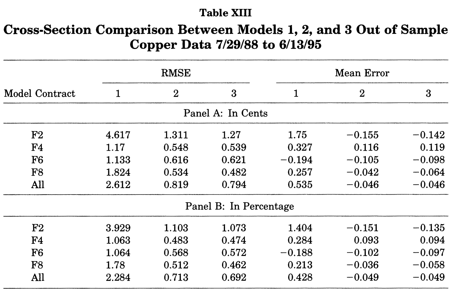
Figure 6.1: Out of sample means for maturities not used at the estimation stage. F1 contract : the closest to maturity F2 : the second contract to maturity and so one. Source: Schwartz (1997).

6.2 Interest-rate swaps and forward contracts

6.2.1 Swap rates

Definition 6.1 (Interest Rate Swap (IRS)) In an Interest Rate Swap (IRS), a fixed-rate payer agrees to provide the fixed-rate receiver with a sequence of cash flows that are determined at the negotiation date of the swap, and at predetermined dates. These cash flows constitute the fixed leg of the swap. Conversely, the fixed-rate receiver provides the fixed-rate payer with cash-flows that depend on future values of a reference rate; this is the floating rate of the swap.

More precisely, the dates of payment are of the form \(t+ \tau\), \(t + 2\tau\), , \(t + n\tau\), where \(\tau\) is a period expressed in years (typically 1/2 or 1/4) and \(n\) is the number of payments. The maturity, or tenor, of the swap contract is \(h = n \tau\).

The payoffs of the fixed leg are \(\tau S\), where \(S\) is the annualized payment (or swap rate). On date \(t+j\tau\), the payoff of the floating leg is \(\tau L(t+(j-1)\tau,\tau)\), where \(L\), the annualized linear rate is given by: \[ L(t+(j-1)\tau,\tau) = \frac{1 - B(t+(j-1)\tau,\tau)}{\tau B(t+(j-1)\tau,\tau)}, \] where \(B(t+(j-1)\tau,\tau)\) is the price, at date \(t+(j-1)\tau\) of a bond of maturity \(\tau\).

On the negotiation date, the values of the fixed and floating legs are identical, so that the value of the swap is zero.

Proposition 6.4 (Swap rate formula) The swap rate \(S(t,h)\), as defined in Def. 6.1 satisfies: \[\begin{equation} \boxed{S(t,h) = \frac{1 - B(t,h)}{\tau \sum_{j=1}^{h/\tau} B(t,j\tau)}.}\tag{6.5} \end{equation}\]

Proof. At \(t\), the price of the fixed leg is: \[ \sum_{j=1}^n \tau S B(t,j\tau). \] Let us turn to the price of the floating leg. The payoff at date \(t+j\tau\), that is \(\frac{1 - B(t+(j-1)\tau,\tau)}{B(t+(j-1)\tau,\tau)}\) is known on date \(t+(j-1)\tau\), so its price at date \(t+(j-1)\tau\) is \(1 - B(t+(j-1)\tau,\tau)\), and its price at \(t\) therefore is \(B(t,(j-1)\tau) - B(t,j\tau)\). Summing over \(j=1,\dots,n\), the date-\(t\) price of the floating leg is \(1 - B(t,n\tau)\) (independent of the payment dates).

Since the price of the contract is zero at date \(t\) (by definition of the swap), we must have: \[ \sum_{j=1}^n \tau S B(t,j\tau) = 1 - B(t,n\tau), \] which gives (6.5).

Note that all the terms appearing in the previous formula are available in closed-form in the context of an affine model (see Example 1.18).

Eq. (6.5) also shows that we have \(100\% = B(t,h) + S(t,h) \tau \sum_{j=1}^{h/\tau} B(t,j\tau)\). This equation means that the swap rate \(S(t,h)\) is homogenous to the yield-to-maturity of a bond valued at par (\(100\%\)), whose coupons are equal to \(S(t,h) \tau\). (The coupons are paid on \(\{t+\tau,\dots,t+n\tau\}\).) In other words, a swap yield is homogenous to a par yield.

6.2.2 Forward rates

Definition 6.2 (Forward Rate Agreement (FRA)) An interest rate forward contract is a contract in which the rate to be paid or received on a specific obligation for a set period, beginning in the future, is set at contract initiation.

Denote by \(f(t,h_1,h_2)\) the forward interest rate, set on date \(t\), for the period between \(t+h_1\) and \(t+h_2\). One of the two counterparties will pay \(\exp(-f(t,h_1,h_2)(h_2 - h_1))\) on date \(t+h_1\), and receive one on date \(t+h_2\).

Proposition 6.1 (Forward rate formula) The forward rate defined in Def. 6.2 satisfies: \[\begin{equation} \boxed{f(t,h_1,h_2) = \frac{h_2 R(t,h_2) - h_1 R(t,h_1)}{h_2 - h_1},}\tag{6.6} \end{equation}\] where \(R_{t,h}\) denotes the date-\(t\) continuously-compounded yield of maturity \(h\).

Proof. Consider two strategies (decided on date \(t\)):

1. Buy a zero-coupon bond of maturity \(h_2\) (price \(B(t,h_2)\)) and sell zero-coupon bonds of maturity \(h_1\) for the same amount (yielding a payoff of \(B(t,h_2)/B(t,h_1)\) on date \(t+h_1\)).
2. Enter a forward rate agreement between dates \(t+h_1\) and \(t+h_2\), whereby you receive 1 on date \(t+h_2\).

These two strategies deliver the same payoffs on date \(t\) (the payoff is zero) and on date \(t+h_2\) (the payoff is 1). By absence of arbitrage, the payoffs on date \(t+h_1\) have to be the same. Therefore \[\begin{eqnarray*} \exp(-(h_2 - h_1)f(t,h_1,h_2)) &=& B(t,h_2)/B(t,h_1) \\ \Rightarrow f(t,h_1,h_2) &=& \frac{1}{h_2 - h_1}(\log[B(t,h_1)] - \log[B(t,h_2)]), \end{eqnarray*}\] which gives (6.6).

In an affine model (where \(R(t,h)\) is an affine function of the state vector \(w_t\)), forward rates are linear in the state vector \(w_t\).