7 Credit and liquidity risks

7.1 Notations

The information of the investor at date \(t\) is still denoted by \(\underline{w_t} = (w_t',w_{t-1}',\dots, w_1 ') '\), but \(w_t\) now comprises a new subsector, namely \(d_t\), that keeps track of the “default” status of some creditors. Formally, \(w_t = (y_t',d_t')'\), where \(y_t\) is a \(n_y\)-dimensional vector of common factors, and \(d_t = (d_{1, t} , \dots, d_{E, t}) '\) a \(E\)-dimensional vector of binary variables representing the possible default of entities \(e \in \{1, \dots,E\}\). Vector \(w_t\) is \(K\)-dimensional, that is \(K = n_y + E\).

By convention:

• \(d_{e, t} = 1\) if entity \(e\) is in default status at time \(t\),
• \(d_{e, t} = 0\) if entity \(e\) is not in default status at time \(t\).

We assume that the process \(\{w_t\}\) is Markov. Formally, its historical (\(\mathbb{P}\)) dynamics is defined by the conditional densities: \[ f (y_t | w_{t-1}) \mbox{ and }p ( d_t | y_t, w_{t-1} ). \]

In what follows, we assume that the default state is absorbing:

Hypothesis 7.1 (absorbing defaults) The default event is an absorbing state. Formally: \(p_e ( 0 | y_t, w_{t-1}, d_{e,t-1}=1 ) = 0\).

The survival probability is defined as follows: \[\begin{equation} p_e ( 0 | y_t, w_{t-1}, d_{e,t-1}=0 ) = \exp[-\underbrace{\lambda_e ( y_t, w_{t-1})}_{\color{blue}{\mbox{default intensity}}}].\tag{7.1} \end{equation}\]

It is easily checked that \(\lambda_e ( y_t, w_{t-1})\) is close to the conditional probability of default when it is small.

7.2 Pricing under standard assumptions

To start with, we will consider the pricing of defaultable bonds under assumptions that are standard in the literature, a framework that we call the classical credit-risk framework. These assumptions—namely 7.2 and 7.3—lead to simple formulas. We will investigate further what happens when these assumptions are relaxed (Subsection 7.4).

Hypothesis 7.2 (Non-systemic entity) \(\{d_t\}\) does not Granger-cause \(\{y_t\}\), in the sense that: \[ f(y_t|w_{t-1}) = f(y_t|y_{t-1}). \]

In other words, under Hypothesis 7.2, \(y_t\) is exogenous to \(d_t\).

Hypothesis 7.3 (Unpriced credit events) The default events (or credit events) are not priced, in the sense that: \[\begin{equation*} \mathcal{M}_{t-1, t}( w_t, w_{t-1}) = \mathcal{M}_{t-1, t}( y_t, y_{t-1}) . \end{equation*}\]

In other words, under Hypothesis 7.3, defaults do not affect the SDF conditionally on \(\underline{y_t}\).

Hypothesis 7.3 also implies that the short-term risk-free rate \(i_t=-\log\mathbb{E}_t(\mathcal{M}_{t,t+1})\) depends on \(\underline{y_t}\) (but not on \(d_t\)).

Figure 7.1 provides a graphical representation of the causality scheme in the classical credit-risk framework.

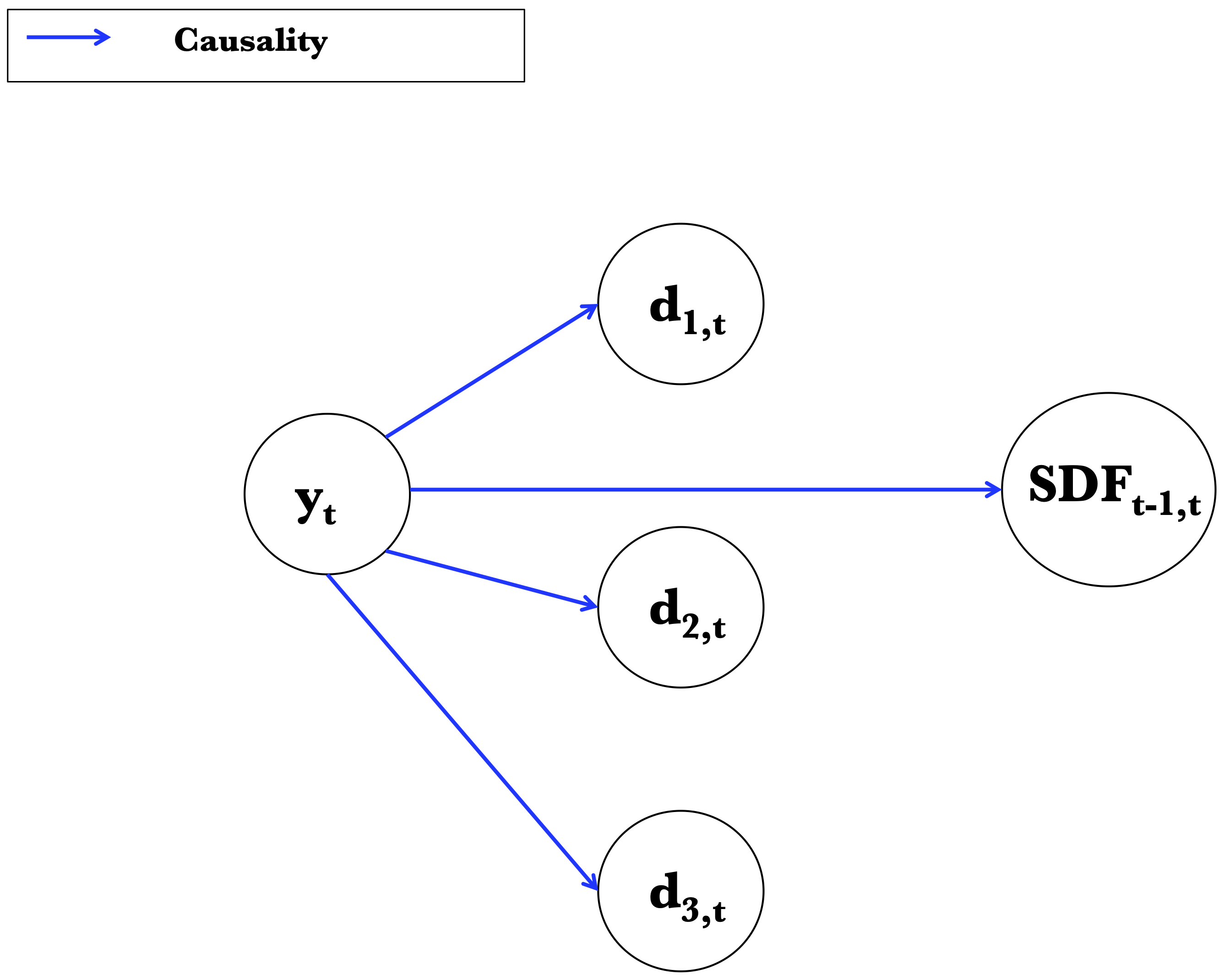
Figure 7.1: Graphical representation of the causality scheme in the classical credit-risk framework.

Proposition 7.1 (Risk-neutral exogeneity of factors) Under Hypotheses 7.2 and 7.3, we have: \[ f^{\mathbb{Q}}(y_t|w_{t-1}) = f^{\mathbb{Q}}(y_t|y_{t-1}), \] that is, \(\{d_t\}\) does not Granger-cause \(\{y_t\}\) under the risk-neutral measure.

Proof. We have: \[\begin{eqnarray} f^{\mathbb{Q}}(y_t|w_{t-1}) &=& f(y_t|w_{t-1})\mathcal{M}_{t-1,t}\exp(i_{t-1})\\ &=& f(y_t|y_{t-1})\mathcal{M}_{t-1,t}\exp(i_{t-1}), \end{eqnarray}\] which gives the results, using that \(\mathcal{M}_{t-1,t}\) and \(\exp(i_{t-1})\) depend on \(y_{t-1}\) only (and not on \(d_t\)).

To simplify, let us focus on a single entity (\(d_t \equiv d_{1,t}\)), alive on date \(t\) (\(d_t=0\)). Consider the date-\(t\) price of a bond issued by the defaultable entity. The residual maturity of this bond is denoted by \(h\), and we consider a zero recovery rate (in case of default, the payoff is zero). Using @ref\tag{2.1}, the price of this bond writes: \[ B^d_{t,h} = \mathbb{E}_t^{\mathbb{Q}}[\exp(-i_t-\dots-i_{t+h-1})(1-d_{t+h})]. \]

The following proposition is at the core of the classical credit-risk framework (Darrell Duffie and Singleton 1999):

Proposition 7.2 (Defaultabe zero-coupon bond pricing in the classical credit-risk framework) Under Hypotheses 7.2 and 7.3, and with a default intensity defined—as in (7.1)—through: \[\begin{equation} \exp[-\lambda_t^{\mathbb{P}}]:=\mathbb{P} ( d_t=0 | \underline{y_{t}}, d_{t-1}=0 ), \end{equation}\] we have: \[\begin{equation} \lambda_t^{\mathbb{Q}} = \lambda_t^{\mathbb{P}}\;(=\lambda_t),\tag{7.2} \end{equation}\] and \[\begin{equation} \boxed{B_{t,h}^d = \mathbb{E}_t^{\mathbb{Q}}\left[\exp\left(-i_t-\dots-i_{t+h-1}- \lambda_{t+1} - \dots - \lambda_{t+h}\right)\right].}\tag{7.3} \end{equation}\] which rewrites, using \(\tilde{i}_t = i_t + \lambda_{t+1}\): \[\begin{equation} B_{t,h}^d = \mathbb{E}_t^{\mathbb{Q}}\left[\exp\left(-\tilde{i}_t-\dots-\tilde{i}_{t+h-1}\right)\right],\tag{7.4} \end{equation}\]

Proof. According to (2.6): \[\begin{equation} f^{\mathbb{Q}}(d_t,y_t|d_{t-1},y_{t-1}) = \exp(i_{t-1})\mathcal{M}_{t-1,t} f^{\mathbb{P}}(d_t,y_t|d_{t-1},y_{t-1}).\tag{7.5} \end{equation}\] Using Hypothesis 7.3, we obtain, by integrating both sides w.r.t. \(d_t\): \[\begin{eqnarray} f^{\mathbb{Q}}(y_t|d_{t-1},y_{t-1}) &=& \exp(i_{t-1})\mathcal{M}_{t-1,t} f^{\mathbb{P}}(y_t|d_{t-1},y_{t-1})\nonumber\\ &=& \exp(i_{t-1})\mathcal{M}_{t-1,t} \underbrace{f^{\mathbb{P}}(y_t|y_{t-1})}_{\mbox{by hypothesis}}. \tag{7.6} \end{eqnarray}\] By Bayes, we have: \[ f^{\mathbb{Q}}(d_t|d_{t-1},y_t,y_{t-1}) = \frac{f^{\mathbb{Q}}(d_t,y_t|d_{t-1},y_{t-1})}{f^{\mathbb{Q}}(y_t|d_{t-1},y_{t-1})}. \] Using (7.5) (numerator) and (7.6) (denominator), we get: \[\begin{eqnarray*} && f^{\mathbb{Q}}(d_t|d_{t-1},y_t,y_{t-1}) = f^{\mathbb{P}}(d_t|d_{t-1},y_t,y_{t-1}), \end{eqnarray*}\] which gives (7.2).

Conditioning w.r.t. \(\underline{y_{t+h}}\), the bond price is given by: \[\begin{eqnarray*} && \mathbb{E}_t^{\mathbb{Q}}[\mathbb{E}_t^{\mathbb{Q}}\{\exp(-i_t-\dots-i_{t+h-1})(1-d_{t+h})|\underline{y_{t+h}}\}]\\ &=& \mathbb{E}_t^{\mathbb{Q}}[\exp(-i_t-\dots-i_{t+h-1})\mathbb{E}_t^{\mathbb{Q}}\{(1-d_{t+h})|\underline{y_{t+h}}\}]\\ &=& \mathbb{E}_t^{\mathbb{Q}}[\exp(-i_t-\dots-i_{t+h-1})\mathbb{Q}\{d_{t+h}=0|\underline{y_{t+h}}\}]\\ &=& \mathbb{E}_t^{\mathbb{Q}}\left[\exp(-i_t-\dots-i_{t+h-1})\prod_{j=1}^h\mathbb{Q}\{d_{t+j}=0|d_{t+j-1}=0,\underline{y_{t+h}}\}\right], \end{eqnarray*}\] Because Granger and Sims non-causalities are equivalent, and since \(d_t\) does not Granger-cause \(y_t\) under the risk-neutral measure (see Proposition 7.1), we have: \[ \mathbb{Q}\{d_{t+j}=0|d_{t+j-1}=0,\underline{y_{t+{\color{red}h}}}\} = \underbrace{\mathbb{Q}\{d_{t+j}=0|d_{t+j-1}=0,\underline{y_{t+{\color{red}j}}}\}}_{=\exp(-\lambda_{t+j}^{\mathbb{Q}})}. \] As a result: \[\begin{equation} B_{t,h}^d = \mathbb{E}_t^{\mathbb{Q}}\left[\exp\left(-i_t-\dots-i_{t+h-1}- \lambda_{t+1}^{\mathbb{Q}} - \dots - \lambda_{t+h}^{\mathbb{Q}}\right)\right].\tag{7.7} \end{equation}\] Using (7.2) in (7.7), we obtain (7.3).

Although \(\mathbb{P}\) and \(\mathbb{Q}\) intensities are the same functions of \(y_t\) and \(y_{t-1}\), their historical and risk-neutral dynamics are in general different since \(y_t\)’s \(\mathbb{P}\) and \(\mathbb{Q}\) dynamics are different.

Eq. (7.4) is reminiscent of (1.10), where the risk-free short-term rate \(i_t\) is replaced by the credit-adjusted short-term rate \(\tilde{i}_t\).

Importantly, if both \(i_t\) and \(\lambda_t\) are affine in \(y_t\), where the latter is an affine process, then bond prices are easily computed by means of recursive formulas (as was the case in the context of (1.10), see Example 1.18.

In this case, \(B_{t,h}^d\) is exponential affine in \(y_t\), that is, it is of the form: \[\begin{equation} B_{t,h}^d = \exp({A^d_h}'y_t + B^d_h)\quad (say).\tag{7.8} \end{equation}\]

The previous framework can be adapted in order to accommodate non-zero recovery rates. In this framework, the default intensity will be replaced by a pseudo, or recovery-adjusted default intensity denoted by \(\tilde\lambda_t\). To go further, we need to specifiy the payoff taking place upon default. There exist different modelling conventions for that; one is the so-called Recovery of Market Value (RMV) (Darrell Duffie and Singleton 1999). Loosely speaking, under the RMV, the recovery payoff is a fraction \(\zeta \in [0,1]\), called Recovery Rate (RR) of the price that would have prevailed, absent the default. Proposition 7.3 makes this definition more precise and gives the bond price stemming from it.

Proposition 7.3 (Bond pricing in the RMV classical framework) Under Hypotheses 7.2 and 7.3, and if, in case of default on date \(t+i\), the recovery payment is \(\zeta \widetilde{B}_{t+i,h-i}\), with \(\zeta \in [0,1]\), then \[\begin{equation} B_{t,h}^d = (1-d_t)\widetilde{B}_{t,h},\tag{7.9} \end{equation}\] where \(\widetilde{B}_{t,h}\) is a pseudo-price given by: \[\begin{equation} \widetilde{B}_{t,h} = \mathbb{E}_t^{\mathbb{Q}} [\exp(-i_{t}-\tilde\lambda_{t+1}-\dots -i_{t+h-1}-\tilde\lambda_{t+h}],\tag{7.10} \end{equation}\] where the pseudo-intensity \(\tilde\lambda_{t}\) is defined by: \[\begin{eqnarray} \exp(-\tilde\lambda_{t+1}) &=& \mathbb{E} [\{1 - d_{t+1} (1-\zeta)\}|\underline{y_{t+1}},d_t=0] \nonumber\\ &=& 1 - (1-\zeta) (1-\exp(-\lambda_{t+1})).\tag{7.11} \end{eqnarray}\]

Proof. Relation (7.9) is true for \(B_{t+h,0}^d\) since \(\widetilde{B}_{t+h,0} = 1\) and \(B_{t+h,0}^d = 1 - d_{t+h}\). Assuming that \(B_{t+i+1, h-i-1}^d = (1 - d_{t+i+1} ) \widetilde{B}_{t+i+1,h-i-1}\) (which is valid for \(i=h-1\)), we get: \[\begin{eqnarray*} B_{t+i, h-i}^d &=& \left(1 - d_{t+i} \right) \mathbb{E}_{t+i}^{\mathbb{Q}} \left\{ \exp(- i_{t+i}) \left[ \left(1 - d_{t+i+1} \right) \widetilde{B}_{t+i+1,h-i-1} \right. \right. \\ && \left. \left. + d_{t+i+1}\zeta\widetilde{B}_{t+i+1,h-i-1} \right] \right\}, \end{eqnarray*}\] since, in case of no default at date \(t+i\), the value of the bond at date \(t+i+1\) is either \(\zeta B_{t+i+1, h-i-1}^d = \zeta \widetilde{B}_{t+i+1,h-i-1}\) if default happens, and \(B_{t+i+1, h-i-1}^d = \widetilde{B}_{t+i+1,h-i-1}\) otherwise. Hypotheses 7.2 and 7.3 imply that \(\widetilde{B}_{t+i+1,h-i-1}\) does not depend on \(d_{t+i+1}\) and taking first the conditional expectation given \(w_{t+i}\) and \(y_{t+i+1}\) we obtain: \[\begin{equation} \begin{array}{lll} B_{t+i, h-i}^d &=& \left(1 - d_{t+i} \right) \mathbb{E}_{t+i}^{\mathbb{Q}} \left\{ \exp(- i_{t+i}) \widetilde{B}_{t+i+1,h-i-1} \times \right. \\ && \quad\left. \mathbb{E}^{\mathbb{Q}} \left[ \left(1 - d_{t+i+1} \right) + \zeta d_{t+i+1} | y_{t+i+1}, w_{t+i} \right] \right\} . \end{array}\tag{7.12} \end{equation}\] Using the definition of \(\widetilde{\lambda}_{t}\) (Eq. (7.11)) we get: \[\begin{equation*} \begin{array}{lll} B_{t+i, h-i}^d &=& \left(1 - d_{t+i} \right) \mathbb{E}_{t+i}^{\mathbb{Q}} \left\{ \exp \left( - i_{t+i} - \widetilde{\lambda}_{t+i+1} \right) \widetilde{B}_{t+i+1,h-i-1} \right\}\\ &=& \left(1 - d_{t+i} \right) \widetilde{B}_{t+i,h-i} . \end{array} \end{equation*}\] Therefore it is also true for \(i=0\).

Again, if \(i_t\) and \(\tilde\lambda_t\) are affine combinations of an affine process \(y_t\), then (exponential affine) bond prices are easily computed by means of recursive formulas. This is formalized below.

Hypothesis 7.4 (Affine process) The process \(\{ y_t \}\) is affine under the \(\mathbb{Q}\) measure: \[\begin{equation} \begin{array}{lll} \varphi^{\mathbb{Q}}_{y, t-1} (u_y) = \mathbb{E}^{\mathbb{Q}} \left[\exp( u_y ' y_t ) | \underline{y_{t-1}} \right] = \exp \left[ a^{\mathbb{Q}}_{y} (u_{y}) ' y_{t-1} + b^{\mathbb{Q}}_{y} (u_{y}) \right], \end{array}\tag{7.13} \end{equation}\] and \(i_t\) and \(\widetilde{\lambda}_{e, t}\) are affine in \((y_t, y_{t-1})\), that is (say): \[\begin{eqnarray} i_{t} &=& \omega_0 + \omega_{1} ' y_{t} \\ \widetilde{\lambda}_{e, t} &=& \kappa_{0} + \kappa_{1}' y_t. \end{eqnarray}\]

Proposition 7.4 (Standard affine bond pricing, under RMV convention) Under the Assumptions of Proposition 7.3 and under Hypothesis 7.4, we have, for \(h \ge 1\): \[\begin{equation} B_{t,h}^d = \left(1 - d_{t} \right)\exp(- h[\omega_0 + \kappa_{0}] - \omega_{1} ' y_{t} + A_h'y_t + B_h),\tag{7.14} \end{equation}\] where \(A_h\) and \(B_h\) are given by the following recursive equations: \[\begin{equation} \left\{ \begin{array}{ccl} A_{h} &=& a(u_{h} + A_{h-1}), \\ B_{h} &=& b(u_{h} + A_{h-1}) + B_{h-1}, \\ A_{0} &=& 0,\quad B_{0} = 0, \end{array} \right.\tag{7.15} \end{equation}\] with \(u_1 = -\kappa_{1}\) and \(u_i = -(\kappa_{1} + \omega_{1})\) for \(i>1\).

Proof. The results directly follows from Proposition 7.3.

What precedes has been estiablished under the assumption that the state vector \(w_t\) comprises a single defaultable entity (\(E=1\)). What about when different entities are considered (\(E = 2\))? We can demonstrate that similar pricing formulas are obtained under the assumption of no-contagion (Hypothesis 7.5):

Hypothesis 7.5 (no contagion) There is no instantaneous or lagged contagion between entities, i.e.: \[\begin{equation*} p ( d_t | y_t, w_{t-1} ) = p_1 ( d_{1, t} | y_t, y_{t-1}, d_{1, t-1}) \times p_2 ( d_{2, t} | y_t, y_{t-1}, d_{2, t-1}) . \end{equation*}\]

If Hypothesis 7.5 is not satisfied, for instance, if we have contagion effect from \(e = 1\) towards \(e = 2\): \[\begin{eqnarray*} p(d_t|y_t, w_{t-1} ) &=& p_1 ( d_{1, t} | y_t, y_{t-1}, d_{1, t-1}) \times \\ && p_2 ( d_{2, t} | y_t, y_{t-1}, \color{blue}{d_{1, t}}, \color{blue}{d_{1, t-1}}, d_{2, t-1}), \end{eqnarray*}\] then:

1. Proposition 7.3 is still valid for both entities;
2. In an affine framework, the computation of \(\widetilde{B}^{(1)}_{t,h}\) (and \(B^{(1)}_{t,h}\)) is straightforward;
3. but formulas for \(\widetilde{B}^{(2)}_{t,h}\) and \(B^{(2)}_{t,h}\) are not explicit anymore even if \(\widetilde{\lambda}_{2, t}\) is affine in \((y_t, y_{t-1}, d_{1, t}, d_{1, t-1})\).

Proposition 7.5 (Absence of contagion) Under Hypotheses 7.1, 7.2, 7.3 and 7.5, the risk-neutral (\(\mathbb{Q}\)) dynamics is such that: \[ f^{\mathbb{Q}} ( y_t | w_{t-1}) = f^{\mathbb{Q}} ( y_t | y_{t-1}) \propto \mathcal{M}_{t-1, t}( y_t, y_{t-1}) f (y_t | y_{t-1}) \] (exogeneity of \(y_t\) preserved under \(\mathbb{Q}\)) and

\[ p_t^{\mathbb{Q}} ( d_{t} | y_t, w_{t-1} ) = p_1 ( d_{1, t} | y_t, y_{t-1}, d_{1, t-1} ) \times p_2 ( d_{2, t} | y_t, y_{t-1}, d_{2, t-1}), \] (absence of contagion preserved under \(\mathbb{Q}\)).

Denoting by \(\lambda^{\mathbb{Q}}_e \left( y_t, y_{t-1} \right) \equiv - \log \left[ p_e^{\mathbb{Q}} ( 0 | y_t, y_{t-1}, 0 ) \right]\) the risk-neutral default intensity of entity \(e\), it comes that: \[ \lambda^{\mathbb{Q}}_e \left( y_t, y_{t-1} \right) = \lambda_e \left( y_t, y_{t-1} \right) \] (default intensities are the same under \(\mathbb{P}\) and \(\mathbb{Q}\)).

Proof. The \(\mathbb{Q}\) conditional density of \(w_t\) given \(w_{t-1}\), namely \(f^{\mathbb{Q}} (y_t | w_{t-1}) p^{\mathbb{Q}} ( d_t | y_t, w_{t-1} )\), is proportional to \(\mathcal{M}_{t-1, t}( w_t, w_{t-1}) f (y_t | w_{t-1}) p ( d_t | y_t, w_{t-1} )\), and thus proportional to \(\mathcal{M}_{t-1, t}( y_t, y_{t-1}) f (y_t | y_{t-1}) p_1 ( d_{1, t} | y_t, y_{t-1}, d_{1, t-1}) p_2 ( d_{2, t} | y_t, y_{t-1}, d_{2, t-1})\). The result follows immediately.

7.3 Pricing illiquid bonds

This subsection shows that a similar approach can be used to price illiquid assets. The idea consists in replacing the Loss Given Default (\(LGD = 1-RR^{(e)}\)) by a Loss Given Liquidity Shock (\(1-\theta_\ell^{(e)}\)). A structural interpretation of this approach is provided by Ericsson and Renault (2006) (see Example 7.1).

Let us introduce a novel binary variable: \(\ell_t\), that represents a liquidity shocks. When a bondholder is hit by the liquidity shock, she needs to liquidate her portfolio (reflecting cash constraints or needs to rebalance portfolio). But in such distressed conditions, she will sell her bonds at a discount (and will therefore face losses, akin to credit losses). Formally: \(\ell_{t}=1\) when the bondholder is hit, and \(\ell_{t}=0\) otherwise.

The liquidity-shock intensity \(\lambda_\ell(y_t)\)—that defines the probability of occurence of liquidity shocks—is defined through: \[ \underbrace{1- \exp[-\lambda_\ell(y_t)]}_{\approx \lambda_\ell(y_t)\mbox{ if small}} = \mathbb{P}(\ell_t = 1|\underline{w_{t-1}},y_t). \] The binary variable \(\ell_t\) is assumed not to Granger-cause \(y_t\) (as in Hypothesis 7.2) and not to be priced (as in Hypothesis 7.3). As in Proposition 7.2—and more precisely equation (7.2)—this implies that \[ \lambda_\ell^{\mathbb{Q}}(y_t) = \lambda_\ell(y_t), \] where \[ 1- \exp[-\lambda^{\mathbb{Q}}_\ell(y_t)] = \mathbb{Q}(\ell_t = 1|\underline{w_{t-1}},y_t). \]

Upon the arrival of the liquidity shock (\(\ell_{t}=1\)), the investor has to exit by selling her bond holdings. She is then limited in the number of traders she can call and, as a result, get only a fraction, \(\theta_\ell^{(e)}\) (say), of the price she would get in normal-liquidity times, i.e., when \(\ell_{t}=0\). Example 7.1 proposes a structural interpretation for \(\theta_\ell^{(e)}\).

In that context, following the approach used in Proposition 7.3, one can define a pseudo-illiquidity intensity as follows—mimicking (7.11): \[\begin{eqnarray} \widetilde{\lambda}_{e,\ell, t} \left( y_t, y_{t-1} \right) &=& - \log \left\{ \exp \Big[ - \lambda_{e,\ell} \left( y_t\right) \Big] \right. + \tag{7.16}\\ && \left. \Big( 1 - \exp \Big[ - \lambda_{e,\ell} \left( y_t \right) \Big] \Big) \theta_\ell^{(e)} \right\}. \nonumber \end{eqnarray}\]

Still consiering credit risk (on top of liquidity risk), we then have the following payoff on date \(t\) (assuming no default on date \(t-1\)): \[\begin{equation} \widetilde{B}^{(e)}_{t,h} = \mathbb{E}^{\mathbb{Q}}_t \left\{ \exp \left[ - \sum_{i=1}^{h} \left( i_{t+i-1} + \widetilde{\lambda}_{e,c, t+i} + \widetilde{\lambda}_{e,\ell, t+i} \right) \right] \right\}.\tag{7.17} \end{equation}\]

Example 7.1 (Structural interpretation of the illiquidity intensity) This structural interpretation of the illiquidity intensity is due to Ericsson and Renault (2006).

When hit by a liquidity shock, a bondholder has to liquidate her bond in a small amount of time (between \(t\) and \(t+\varepsilon\), with \(\varepsilon \ll 1\)). She collects a random number (\(\kappa\)) of offers on the market. This number follows a Poisson distribution of parameter \(\varepsilon\gamma^{(e)}\); the more liquid the bond, the higher \(\gamma^{(e)}\). Each offer is a random fraction \(\omega_{i}\) (\(i\in\{1,\ldots,\kappa\}\)) of \(\widetilde{B}^{(e)}_{t,h}\) (see Eq. (7.17)), where the \(\omega_{i}\)’s are independently and uniformly distributed in \([0,1]\).

At \(t+\varepsilon\), the bond is sold to the trader that has offered the highest price. Formally, when \(\ell_{t}=1\), the selling price is: \[ \left(\max_{i\in\{1,\ldots,\kappa\}}\omega_{i}\right)\tilde{P}_{t,h}^{(e)}, \quad \mbox{with}\quad \kappa \sim \mathcal{P}(\varepsilon\gamma^{(e)}). \] Conditional on \(\kappa\), the expectation of \(\max_{i}(\omega_{i})\) is \(\kappa/(\kappa+1)\). (Because the \(\omega_{i}\) are i.i.d., the c.d.f. of \(\max(\omega_{1},\ldots,\omega_{\kappa})\) is \(x\mapsto F(x)^{\kappa}\), where \(F\) is the c.d.f. of \(\omega_{i}\).) Hence, \(\theta_\ell^{(e)}\)—the unconditional expectation of \(\max_{i}(\omega_{i})\)—is given by: \[\begin{eqnarray*} \sum_{k=1}^{\infty}\frac{e^{-\varepsilon\gamma^{(e)}}k}{k+1}\frac{\left(\varepsilon\gamma^{(e)}\right)^{k}}{k!} & = & \left[\left(1-e^{-\varepsilon\gamma^{(e)}}\right)\frac{\varepsilon\gamma^{(e)}-1}{\varepsilon\gamma^{(e)}}+e^{-\varepsilon\gamma^{(e)}}\right]\\ & = & g(\varepsilon\gamma^{(e)})\qquad\mbox{(say).} \end{eqnarray*}\] Function \(g\) is increasing and valued in \([0,1]\). In addition \(\lim_{x\rightarrow\infty}g(x)\rightarrow1\).

The scalar \(g(\varepsilon\gamma^{(e)})\) can be seen as the structural interpretation of the parameter \(\theta_\ell^{(e)}\), which is discussed in the present section.

Example 7.2 (Euro area sovereign credit spreads) A. Monfort and Renne (2011) and Alain Monfort and Renne (2014) propose credit/liquidity decompositions of euro-area sovereign spreads. They emply different estimation approaches: C.-J. Kim (1994)’s filter for MR2014, and Kitagawa-Hamilton filter for A. Monfort and Renne (2011) (see Subsection 5.3.1).

In both papers, the \(y_t\) part of the state vector \(w_t\) is of the form \(y_t = (x_t',z_t')'\); it follows a Regime-Switching Gaussian VAR (see Example 5.3). The time-homogenous Markov chain \(z_t\) tracks the crisis status (crisis versus normal times).

The total intensity is of the form: \[ \widetilde{\lambda}_{e,t} = \underbrace{\alpha_{e,c}'z_t + \beta_{e,c}'y_t}_{\mbox{credit intensity $\widetilde{\lambda}_{e,c,t}$}} + \underbrace{\alpha_{e,\ell}'z_t + \beta_{e,\ell}'y_t.}_{\mbox{liquidity intensity $\widetilde{\lambda}_{e,\ell,t}$}} \] In both papers, the identification of credit versus liquidity components is based on: \[ \mbox{KfW-Bund spreads} = \mbox{liquidity spreads}. \] KfW (Kreditanstalt für Wiederaufbau) is a German agency whose bonds are guaranteed by the Federal Republic of Germany. Therefore, they benefit from the same credit quality than their sovereign counterparts—the Bunds—but are less liquid; accordingly, the KfW-Bund spread should beessentially liquidity-driven.

In Alain Monfort and Renne (2014), we have \[ \widetilde{\lambda}_{e,t} = \underbrace{x_{e,t}}_{=\widetilde{\lambda}_{e,c,t}} + \underbrace{(1-\theta^{(e)}_\ell)x_{E+1,t}}_{=\widetilde{\lambda}_{e,\ell,t}}, \] hence \(x_t\) of dimension \(E+1 = 12\) (11 countries are involved).

There are 9 Markovian regimes: \(z_t = z_{c,t} \otimes z_{\ell,t}\), where \(z_{i,t}\) (\(i \in \{c,\ell\}\)) is 3-dimensional:

• \(z_{i,t}=[1,0,0]'\): low stress,
• \(z_{i,t}=[0,1,0]'\): medium stress,
• \(z_{i,t}=[0,0,1]'\): high stress.
• \(z_{c,t}\) and \(z_{\ell,t}\) are not independent: for instance, the probability to transit from the low-credit-stress regime to the medium/high-credit-stress regimes depends on the liquidity-stress regime.

The dynamics of each intensity \(x_{i,t}\) is as follows: \[ x_{i,t} = \mu_i'z_t + \phi x_{i,t-1} + \sigma_i \varepsilon_{i,t}, \] with \(\varepsilon_{t} \sim i.i.d. \mathcal{N}(0,\Sigma)\), where \(\Sigma\) is diagonal, and \(\mu_{i,1} < \mu_{i,2} < \mu_{i,3}\). The Markov chain \(z_t\) is the only source of correlation across the \(x_{i,t}\)’s.

Figure 7.2 shows a simulation of such a process, with: \[ \mu=\left[\begin{array}{c} 0.01 \\ 0.03 \\ 0.10\end{array}\right],\quad \phi=.8 ,\quad P=\left[\begin{array}{ccc} 0.98 & 0.02 & 0\\ 0.05 & 0.90 & 0.05\\ 0 & 0.20 & 0.80 \end{array}\right],\quad \sigma = 0.002. \]

The SDF exponential affine in \((z_t',x_t')'\). We have the same type of dynamics under \(\mathbb{Q}\) (with risk-asjusted parameters, in particular risk-adjusted transition probabilities).

Figure 7.2: Simulation of an process following \(x_{t} = \mu'z_t + \phi x_{t-1} + \sigma \varepsilon_{t}\), where \(z_t\) follows a three-state time-homogenous Markov process. See the text for the exact parameterization. The light-grey shaded area corresponds to the second regime (\(z_t = [0,1,0]'\)); the dark-grey shaded area corresponds to the third regime (\(z_t = [0,0,1]'\))

Example 7.3 (IBOR-OIS spreads) Dubecq et al. (2016) decompose the EURIBOR versus Overnight Index Swap (OIS) spreads into a credit and a liquidity component. (See Subsection 6.2.1 for the definition of a swap contract.)

From the point of view of bank \(j\), the EURIBOR rate is the rate of an unsecured loan to one bank (\(e\), say) of the panel. Assume that the panel of the \(N\) constituting the EURIBOR are homogenous. We have: \[\begin{equation} R^{IBOR}_{t,h} = - \frac{1}{h} \log \mathbb{E}^{\mathbb{Q}}_t \left\{ \exp \left[ - \sum_{i=1}^{h} \left( i_{t+i-1} + \widetilde{\lambda}_{e,c, t+i} + \widetilde{\lambda}_{j,\ell, t+i} \right) \right] \right\}.\tag{7.18} \end{equation}\] Note that the liquidity intensity refers to the lending bank (\(j\)) and the default intensity relates to the borrowing bank (\(e\)).

By constrast, the Overnight-Index Swap (OIS) rate satisfies:²³ \[\begin{equation} R^{OIS}_{t,h} = - \frac{1}{h} \log \mathbb{E}^{\mathbb{Q}}_t \left\{ \exp \left( - \sum_{i=1}^{h} i_{t+i-1} \right) \right\}.\tag{7.19} \end{equation}\]

Assuming that \(i_t\), the short-term risk-free rate (i.e., the reference rate of the OIS, EONIA here) is independent from the intensities and under the homogeneity assumption, we obtain:²⁴ \[ R^{IBOR}_{t,h} - R^{OIS}_{t,h} = - \frac{1}{h} \log \mathbb{E}^{\mathbb{Q}}_t \left\{ \exp \left[ - \sum_{i=1}^{h} \left( \widetilde{\lambda}_{c, t+i} + \widetilde{\lambda}_{\ell, t+i} \right) \right] \right\}. \]

Dubecq et al. (2016) employ a quadratic specification for \(\widetilde{\lambda}_{c, t}\) and \(\widetilde{\lambda}_{\ell, t}\): \[ \widetilde{\lambda}_{c, t} = x_{c,t}^2 \quad \mbox{and} \quad \widetilde{\lambda}_{\ell, t} = x_{\ell,t}^2, \] where \(X_t = (x_{c,t},x_{\ell,t})'\) follows a Gaussian VAR(1) process. (This is the quandratic Gaussian framework presented in Example 1.7.)

The state vector \(X_t\) is latent. The estimation involves the Quadratic Kalman Filter (Alain Monfort, Renne, and Roussellet 2015). The measurement equations include equations stating that observed proxies of credit and liquidity risks relate to quadratic functions of \(x_{c,t}\) and \(x_{\ell,t}\), respectively.

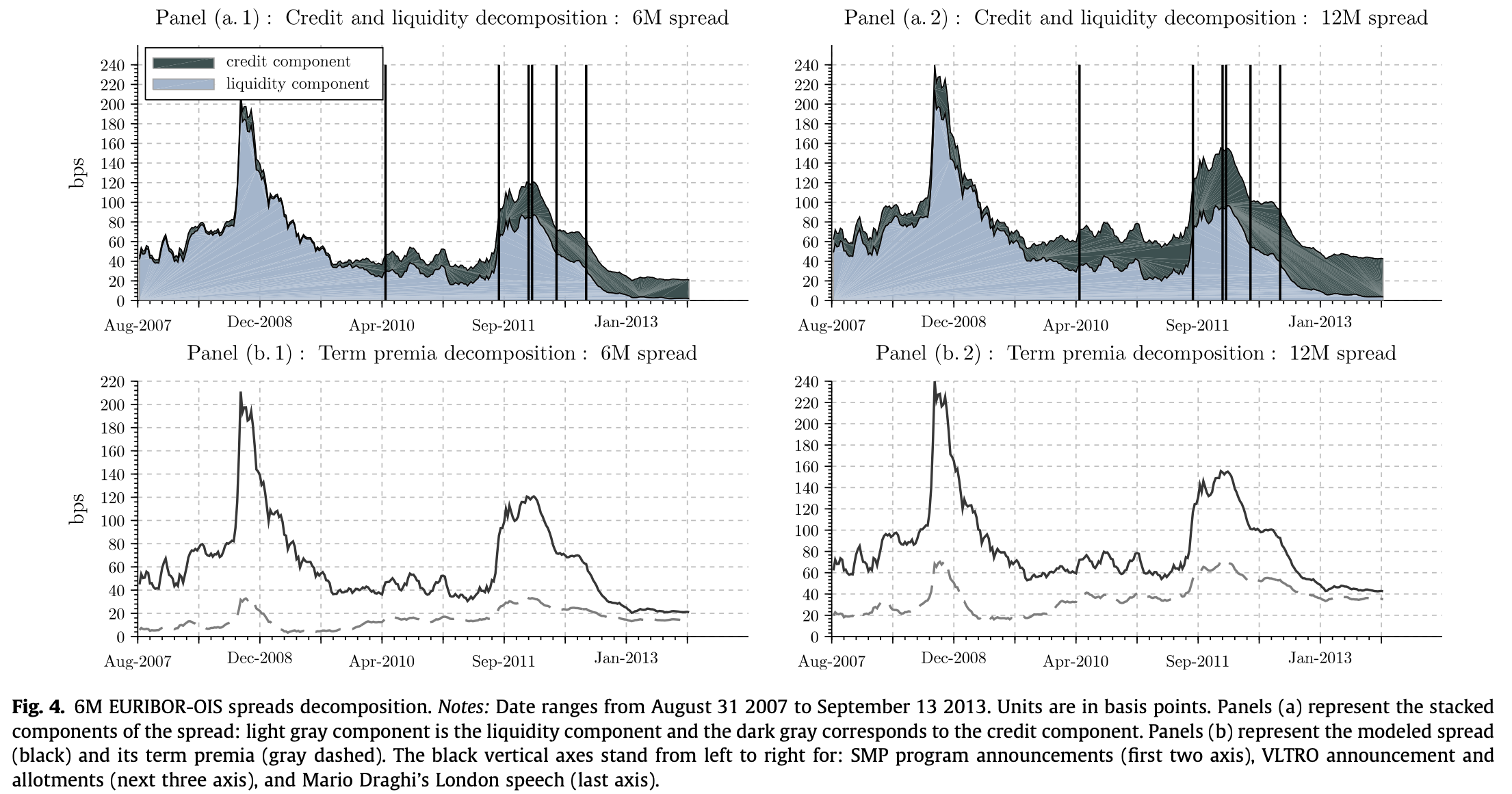
Figure 7.3: Source: Dubecq et al. (2016).

7.4 Relaxing the classical framework assumptions

Formula (7.14) and its tractability is a key feature of numerous credit-risk term-structure models, e.g., D. Duffie and Singleton (2003), Pan and Singleton (2008), and Longstaff et al. (2011) among many others. This formula is valid under Assumptions 7.2 of non-systemic entities, also called no-jump condition, 7.3 of unpriced credit risk events, and 7.5 absence of contagion. These hypotheses define what we have called the classical credit-risk models. We lose the high degree of tractability of Formula (7.14) when some of the previous assumptions are relaxed:

• If \(f (y_t | w_{t-1}) = f (y_t | y_{t-1} , d_{1, t-1})\) (entity \(e = 1\) is systemic) then:

  1. The pseudo-price \(\widetilde{B}^{(e)}_{t,h}\) now depends on \(y_t\) and \(d_{1, t}\);
  2. Eq. (7.3) is valid for entity \(e = 2\) only;
  3. The computation of \(\widetilde{B}^{(2)}_{t,h}\) is not straightforward: \(\{ y_t \}\) is not autonomous and the autonomous process \(\{ y_t, d_{1,t} \}\) is not affine.

• If there is a contagion effect from \(e = 1\) towards \(e = 2\), i.e., if \[\begin{eqnarray*} p ( d_t | y_t, w_{t-1} ) &=& p_1 ( d_{1, t} | y_t, y_{t-1}, d_{1, t-1}) \\ && p_2 ( d_{2, t} | y_t, y_{t-1}, d_{1, t}, d_{1, t-1}, d_{2, t-1}), \end{eqnarray*}\] then:

  1. Eq. (7.3) is still valid for both entities;
  2. In an affine framework, the computation of \(\widetilde{B}^{(1)}_{t, h}\) (and \(B^{(1)}_{t,h}\)) is straightforward; but formulas for \(\widetilde{B}^{(2)}_{t,h}\) and \(B^{(2)}_{t,h}\) are not explicit anymore even if \(\widetilde{\lambda}_{2, t}\) is affine in \((y_t, y_{t-1}, d_{1, t}, d_{1, t-1})\).

• If the default event of the first entity only (\(d_{1,t}\)) is a source of risk that is priced: \(\mathcal{M}_{t-1, t}( w_t, w_{t-1}) = \mathcal{M}_{t-1, t}( y_t, y_{t-1}, d_{1, t}, d_{1, t-1})\), then

  1. \(\lambda^{\mathbb{Q}}_{1, t} \neq \lambda_{1, t}\) and \(\lambda^{\mathbb{Q}}_{2, t} = \lambda_{2, t}\);
  2. the exogeneity of \(\{ y_t \}\) is no longer preserved under \(\mathbb{Q}\);
  3. Eq. (7.3) is no longer valid for entity \(e = 1\). It remains valid for \(e=2\) but the computation of \(\widetilde{B}^{(2)}_{t,h}\) is not straightforward: even if \(y_t\) is \(\mathbb{P}\)-autonomous, this is not true under \(\mathbb{Q}\).

7.4.1 General affine credit-risk framework

Exploiting Vector Auto-Regressive Gamma (VARG) processes, Alain Monfort et al. (2021) propose a general affine credit-risk pricing model jointly allowing for:

1. systemic entities (breaking down the no-jump condition; see Collin-Dufresne, Goldstein, and Hugonnier (2004));
2. contagion effects between entities (economic/financial linkages; see Ait-Sahalia, Laeven, and Pelizzon (2014));
3. pricing of credit events (credit spread puzzle; see C. Gourieroux, Monfort, and Renne (2014));
4. and stochastic recovery rates (RR) (Altman et al. 2005).

In this general framework, the state vector \(w_t\) is of the form \([y_t',\delta_t']'\), where \(\delta_t\) is a \(E\)-dimensional vector of credit-event variables (see Hypothesis 7.6).

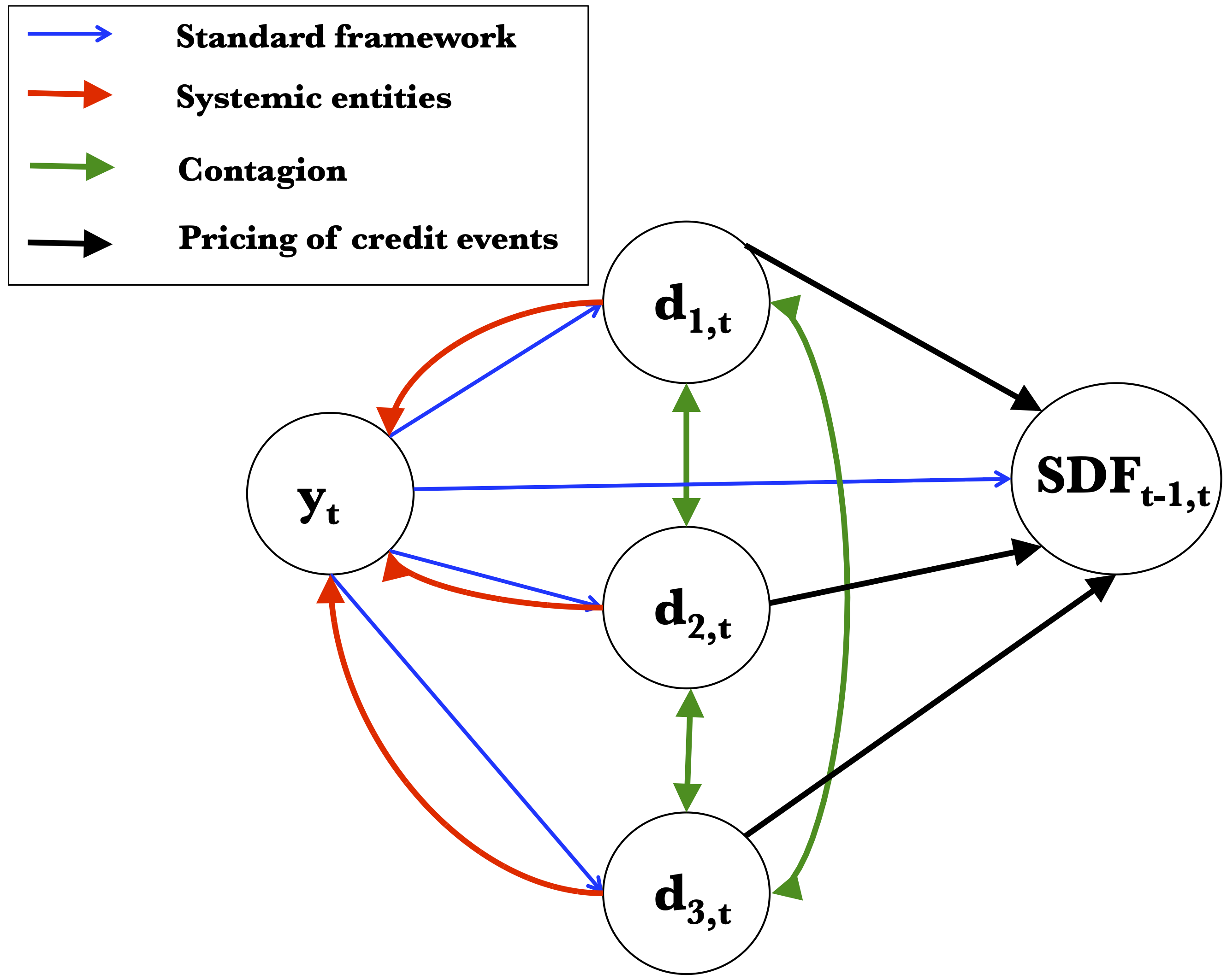
Figure 7.4: Schematic comparison of the classical and general credit-risk frameworks.

Hypothesis 7.6 (Credit events) The default date \(\tau^{(e)}\) (say) of any entity \(e\) is defined as: \[\begin{equation} \tau^{(e)} = \inf \left\{ t > 0 : \delta^{(e)}_t > 0 \right\},\tag{7.20} \end{equation}\] where \(\delta^{(e)}_t\) is a non-negative variable called credit-event variable. The default indicator function can be equivalently written as \(d^{(e)}_t = \textbf{1}_{ \{ \tau^{(e)} \leq t \} }\) or \(d^{(e)}_t = 1 - \textbf{1}_{ \{ \underline{\delta^{(e)}_t} ' {\bf 1} = 0 \} }\), with \(\underline{\delta^{(e)}_t} = (\delta^{(e)}_t, \ldots, \delta^{(e)}_1)\) and where \({\bf 1} = (1, \ldots, 1)'\) with conformable dimension.

Hypothesis 7.7 (State-vector dynamics) The stochastic process \(\{w_t\}\) is affine under the historical probability measure \(\mathbb{P}\). The historical Laplace transform of \(w_t\), conditional \(\underline{w}_{t-1}\), is denoted by: \[\begin{eqnarray} \varphi^{\mathbb{P}}_{w, t-1} (u_w) &=& \mathbb{E} \left[\exp( u_w ' w_t ) | \underline{w_{t-1}} \right] \nonumber \\ &=& \exp \left[ a_{w} (u_{w}) ' w_{t-1} + b_{w} (u_{w}) \right],\tag{7.21} \end{eqnarray}\] with \(u_w = (u_y ', u_{\delta} ')'\).

Example 7.4 (Vector Autoregressive Gamma process) In Alain Monfort et al. (2021), \(w_t\) follows a VARG (positive affine) process, which satisfies Hypthesis 7.7 (Example 1.8 presents the univariate version of this process.): \[\begin{equation} \begin{array}{lll} y_{t} | \underline{w_{t-1}} &\overset{\mathbb{P}}{\sim}& \otimes_{j=1}^{N_y} \gamma_{\nu_{j}^{(y)}} \left( \alpha_{j}^{(y)} + \overbrace{\beta_{j, y}^{(y)} y_{t-1}}^{\mbox{factors}} + \underbrace{ \overbrace{\color{blue}{ \beta^{(y)}_{j, \delta} \delta_{t-1}}}^{\begin{array}{c}\mbox{credit-event}\\\mbox{variables}\end{array}}}_{\begin{array}{c}\color{red}{\mbox{kills no-jump}}\\\color{red}{\mbox{condit.}}\end{array}} , \mu_j^{(y)} \right) \\ \delta_t | y_t, \underline{w_{t-1}} &\overset{\mathbb{P}}{\sim}& \otimes_{e = 1}^{E} \gamma_{0} \left( \alpha_e^{(\delta)} + \color{blue}{\beta^{(\delta)}_{e, y} y_{t}} + \underbrace{\color{blue}{\beta^{(\delta)}_{e, \delta} \delta_{t-1}}}_{\color{red}{\mbox{contagion}}}, \mu_e^{(\delta)} \right) , \end{array}\tag{7.22} \end{equation}\] where \(\delta_t = (\delta^{(1)}_t, \ldots, \delta^{(E)}_t)'\) and \(\gamma_{\nu} \left(\lambda, \mu \right)\): non-central Gamma distribution.

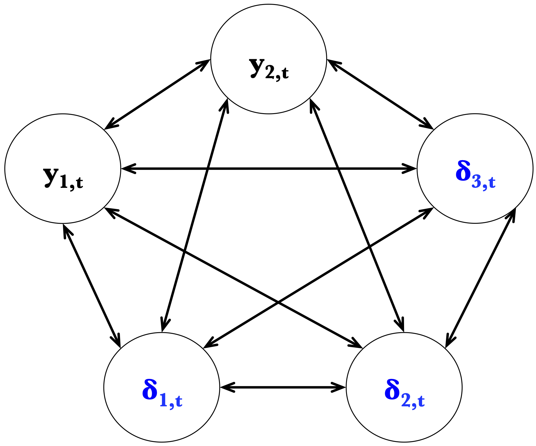
Figure 7.5: A potential causality scheme in Monfort et al. (2021).

Hypothesis 7.8 (Stochastic discount factor) The one-period positive SDF \(\mathcal{M}_{t-1, t}\) is given by (this is (2.4), with \(\alpha_t \equiv \alpha_w\)): \[\begin{equation} \mathcal{M}_{t,t+1} = \exp[-i_{t}+\alpha'_w w_{t+1}-\psi_t(\alpha_w)], \end{equation}\] where \(\alpha_w = (\alpha_y ' , \alpha_x ' , \alpha_{\delta} ') '\) is the vector of prices of risk, and the risk-free short rate (between \(t\) and \(t+1\)) is given by the following affine function of the factors: \[\begin{equation} \begin{array}{lll} i_{t}(\underline{w_{t}}) = \xi_0 + \xi_1 ' w_{t}. \end{array}\tag{7.23} \end{equation}\]

Under Hypotheses 7.7 and 7.8, it comes that: \[\begin{eqnarray} \varphi^{\mathbb{Q}}_{w, t-1} (u_w) &=& \mathbb{E}^{\mathbb{Q}} \left[\exp( u_w ' w_t ) | \underline{w_{t-1}} \right] \nonumber \\ &=& \exp \left[ a^{\mathbb{Q}}_{w} (u_{w}) ' w_{t-1} + b^{\mathbb{Q}}_{w} (u_{w}) \right],\tag{7.24} \end{eqnarray}\] where, using (2.8): \[\begin{equation} \left\{ \begin{array}{ccl} a^{\mathbb{Q}}_{w} (u_{w}) &=& a_{w} (u_{w} + \alpha_w) - a_{w} (\alpha_w) \\ b^{\mathbb{Q}}_{w} (u_{w}) &=& b_{w} (u_{w} + \alpha_w) - b_{w} (\alpha_w). \end{array} \right.\tag{7.25} \end{equation}\]

Hypothesis 7.9 (General recovery payment) The Recovery Paymentof a defaultable ZCB, in the case of default at date \(t+i = \tau^{(e)}\), is given by: \[\begin{equation} \begin{array}{lll} RR^{(e)}_{t+i} \times \mathcal{V}^{(e)}_{t+i, h-i} \end{array}\tag{7.26} \end{equation}\] where the Recovery Rate \(RR^{(e)}_{t+i}\) is \[\begin{equation} RR^{(e)}_{t+i} = \exp \left( - a_{e} - a_{w, e} ' w_{t+i} \right),\tag{7.27} \end{equation}\] and where \(\mathcal{V}^{(e)}_{t+i, h-i}\) denotes the Recovery Value (Exposure-at-Default) at \(t+i\)}.

The general framework allows for flexible specifications of the recovery payment. It can be:

• the fraction of the pre-default value of the claim (Recovery of Market Value, or RMV), see Proposition 7.7;
• the fraction of par (Recovery of Face Value, or RFV), see Proposition 7.6;
• the fraction of a no-default version of the same claim (Recovery of Treasury, or RT). In that case, the recovery payment is a fraction of the (risk-free) present value of the principal.

Proposition 7.6 (General pricing under the RFV convention) The price, at date \(t < \tau^{(e)}\), of a ZCB issued by entity \(e\) and maturing in \(h\) periods is given by: \[\begin{equation} \begin{array}{lll} \boxed{B^{(e)}_{t,h} = \sum_{i = 1}^{h} \left( \Lambda^{\mathbb{Q}}_{(1, t, i)} - \Lambda^{\mathbb{Q}}_{(2, t, i)} \right) + \Lambda^{\mathbb{Q}}_{(3, t, h)} ,} \end{array}\tag{7.28} \end{equation}\] where: \[\begin{equation} \begin{array}{lll} \Lambda_{(1,t,i)}^{\mathbb{Q}} &:=& \underset{u \rightarrow - \infty}{\lim} \Psi^{\mathbb{Q}}_{(t, i)} (a_e , u \widetilde{e}_\delta - \xi_1, - a_{w,e}) \\ \Lambda_{(2,t,i)}^{\mathbb{Q}} &:=& \underset{u \rightarrow - \infty}{\lim} \Psi^{\mathbb{Q}}_{(t, i)} (a_e , u \widetilde{e}_\delta - \xi_1,u \widetilde{e}_\delta - a_{w,e} ) \\ \Lambda_{(3,t,i)}^{\mathbb{Q}} &:=& \underset{u \rightarrow - \infty}{\lim} \Psi^{\mathbb{Q}}_{(t, i)} (0 , u \widetilde{e}_\delta - \xi_1,u \widetilde{e}_\delta) \end{array}\tag{7.29} \end{equation}\] with \(u \in \mathbb{R}\) and where [denoting \(\varphi^{\mathbb{Q}}_{w, t, i} \left(u_2, \ldots, u_2 , u_1 \right) = \varphi^{\mathbb{Q}}_{w, t, i} \left( u_2 , u_1 \right)\)]: \[\begin{equation} \begin{array}{lll} \Psi^{\mathbb{Q}}_{(t, i)} (\kappa , u_1, u_2) &:=& \exp \left[ -i \xi_0 + \kappa + u_2 ' w_t \right] \varphi_{w,t,i}^{\mathbb{Q}}(u_2, u_1) \end{array}\tag{7.30} \end{equation}\]

Proof. See Alain Monfort et al. (2021).

Proposition 7.7 (General pricing under the RMV convention) If the recovery value at date \(t+i\) (defined in 7.9) is of the form: \[\begin{equation} \mathcal{V}^{(e)}_{t+i, h-i} = \mathbb{E}^{\mathbb{Q}} \left\{ \exp \left[ - \sum_{j = i}^{h-1} \left(i_{t+j} + \delta^{(e)}_{t+j+1} \right) \right] \Big| \underline{w_{t+i}} \right\},\tag{7.31} \end{equation}\] with \(RR_t^{(e)} = \exp(-\delta_t^{(e)})\), and under Hypothesis 7.6 to 7.8, the price \(B^{(e)}_{t,h}\) at date \(t < \tau^{(e)}\) is given by: \[\begin{equation} B^{(e)}_{t,h} = \mathcal{V}^{(e)}_{t, h},\tag{7.32} \end{equation}\] where \[\begin{equation} \begin{array}{lll} \mathcal{V}^{(e)}_{t, h} = \exp \left[ \left( \mathcal{A}_h - \xi_1 \right) ' w_t + \left( \mathcal{B}_h - h \xi_0 \right) \right]. \end{array}\tag{7.33} \end{equation}\] where \(\mathcal{A}_h\) and \(\mathcal{B}_h\) are obtained recursively by employing Eqs. (1.19) of Proposition 1.5, replacing functions \(a\) and \(b\) with \(a^{\mathbb{Q}}\) and \(b^{\mathbb{Q}}\) (see Eq. (7.25)) with \(u_{1} = - \widetilde{e}_{\delta}\) and, for \(i>1\), \(u_i = - (\widetilde{e}_{\delta} + \xi_1)\) where \(\widetilde{e}_{\delta} = (0',e_{\delta}')'\) is a \(N\)-dimensional vector, and where \(e_{\delta}\) is the \(e^{th}\) column of the \((N_{\delta}, N_{\delta})\)-dimensional identity matrix.

Proof. See Appendix A.4 of Alain Monfort et al. (2021).

Eq. (7.32) is a key result. It reads: \[\begin{equation} \boxed{B^{(e)}_{t,h} = \mathbb{E}^{\mathbb{Q}} \left\{ \exp \left[ - \left( \sum_{i = 1}^{h}\color{red}{i_{t+i-1} + \delta^{(e)}_{t+i}} \right) \right] \Big| \underline{w_{t}} \right\}.}\tag{7.34} \end{equation}\] It is reminiscent of (7.3), with \(\lambda\) (default intensity) replaced with \(\delta\) (credit-event variable). However, contrary to the classical framework, credit events are priced sources of risk, the no-jump condition is relaxed, contagion is allowed, and the recovery rate is stochastic. This formula can therefore be seen as a generalization of the setting of Darrell Duffie and Singleton (1999).

7.4.2 CDS pricing in the general framework

This subsection shows how CDS can be priced in the context of the general credit-risk model. We consider two types of CDS. The first is the standard one; the second is a CDS whose payoffs are expressed in a foreign currency (which is typical to sovereign CDSs). Figures 7.6 and 7.7 show the payoffs associated with these two types of CDSs.

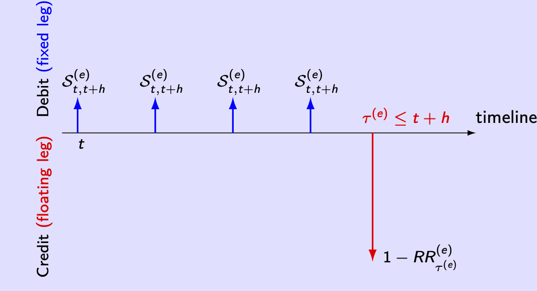
Figure 7.6: CDS payoffs.

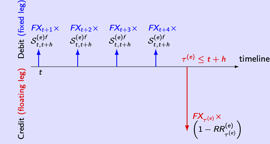
Figure 7.7: CDS payoffs when the payoffs are expressed in a foreign currency.

Since the domestic-currency case is a special case of the multi-currency one, we focus on the latter case in the following.

Pricing a CDS amounts to determining \(\mathcal{S}_{t,t+h}^{(e)}\), that is the CDS spread, for \(t < \tau^{(e)}\). The spread \(\mathcal{S}_{t,t+h}^{(e)}\) is such that the date-\(t\) value of the fixed leg’s payoffs is equal to the date-\(t\) value of the floating leg’s payoffs. The payoffs of the assets issued by the reference entity are assumed to be expressed in the domestic currency.

The (logarithmic) exchange rate is denoted by \(s_t = \ln ( FX_t )\). By convention, an increase in \(s_t\) corresponds to a depreciation of the domestic currency. (In other words, \(FX_t\) is the value of one unit of foreign currency expressed in the domestic currency.) We consider a CDS whose notional is equal to one unit of the foreign currency (i.e. to \(\exp (s_t)\) units of the domestic currency).

Let us determine the value of the fixed leg. If entity \(e\) has not defaulted at date \(t+i\) (\(\le t+h\)), the cash flow on this date, expressed in the domestic currency, is: \[\begin{equation*} \begin{array}{lll} \mathcal{S}^{(e) f}_{t,t+h} \exp(s_{t+i}). \end{array} \end{equation*}\] Hence, the present values of the fixed-leg payments, expressed in the domestic currency are: \[\begin{equation*} \begin{array}{lll} \mathcal{S}^{(e) f}_{t, t+h} \sum_{i=1}^{h} \mathbb{E}^{\mathbb{Q}} \left[\exp \left( s_{t+i} - \sum_{j = 1}^{i} i_{t + j - 1} \right) \textbf{1}_{\{ \delta^{(e) '}_{t : t+i} {\bf 1} = 0 \} } \Big| \underline{w_t} \right], \end{array} \end{equation*}\]

Let us turn to the floating leg. Under the RFV convention, the protection seller will make a payment of \((1 - RR^{(e)}_{t+i}) \exp(s_{t+i})\) (this is the loss-given-default. LGD) at date \(t+i\) in case of default over the time interval \(] t + i - 1, t+i ]\). The present values of the floating leg, expressed in the domestic currency, is: \[\begin{equation*} \begin{array}{lll} && \sum_{i=1}^{h} \mathbb{E}^{\mathbb{Q}} \left[ \exp \left( s_{t+i} - \sum_{j = 1}^{i} i_{t + j - 1} \right) (1 - RR^{(e)}_{t+i})\right. \\ \\ && \hspace{7em} \left. \left( \textbf{1}_{\{ \delta^{(e) '}_{t : t+i-1} {\bf 1} = 0 \} } - \textbf{1}_{\{ \delta^{(e) '}_{t : t+i} {\bf 1} = 0 \} } \right) \Big| \underline{w_t} \right],\tag{7.35} \end{array} \end{equation*}\]

We assume that \(RR^{(e)}_{t} = \exp \left( - a_{e} - a_{w, e} ' w_t \right)\) and that \(s_t = \chi + u_s ' w_t\).

Proposition 7.8 (Price of a multi-currency CDS) In the context described above, we have: \[\begin{equation} \boxed{\mathcal{S}^{(e) f}_{t, t+h} = \frac{\sum_{i=1}^{h} \Lambda^{\mathbb{Q}}_{(t, i)} }{\sum_{i=1}^{h} \lim_{u \to - \infty} \Psi^{\mathbb{Q}}_{(t, i)} \left( \chi, u \tilde{e}_{\delta} - \xi_1 , u \tilde{e}_{\delta} + u_s \right)},}\tag{7.36} \end{equation}\] where: \[\begin{eqnarray*} \Lambda^{\mathbb{Q}}_{(t, i)} & = & \underset{u \to - \infty}{\lim} \Big[ \Psi^{\mathbb{Q}}_{(t, i)} \left( \chi , u \widetilde{e}_{\delta} - \xi_1 , u_s \right) - \Psi^{\mathbb{Q}}_{(t, i)} \left( \chi , u \widetilde{e}_{\delta} - \xi_1 , u \widetilde{e}_{\delta} + u_s \right) \\ && \hspace{7em} - \Psi^{\mathbb{Q}}_{(t, i)} \left(\chi - a_e, u \widetilde{e}_{\delta} - \xi_1 , u_s - a_w \right) \\ && \hspace{7em} + \Psi^{\mathbb{Q}}_{(t, i)} \left(\chi - a_e, u \widetilde{e}_{\delta} - \xi_1 , u \widetilde{e}_{\delta} + u_s - a_w \right) \Big] , \end{eqnarray*}\] and where \(\Psi^{\mathbb{Q}}_{(t, i)} \left(\kappa, u_2 , u_1 \right)\) is given in (7.30).

Proof. See Online Appendix A.4 of Alain Monfort et al. (2021). The proof notably makes use of Lemma 1.2 (Subsection 1.3).

To price a standard CDS (with payments in domestic currency), one simply has to set \(\chi=0\) and \(u_s=0\), which gives \(s_t=0\) (since \(s_t = \chi + u_s ' w_t\)).

Alain Monfort et al. (2021) exploit these formulas to model quanto CDSs in the euro area. Quanto CDSs are spread differentials between the two types of CDS (Augustin, Chernov, and Song 2020). They exploit this framework to estimate “depreciations upon default”. Indeed, in their model, \(s_t\) (the log EURUSD exchange rate) is affected by the credit event variables \(\delta_t\).

7.5 Top-down approach

• Relaxing the assumptions underlying the classical framework can also be done in the context of top-down approaches. Top-down models focus on default counting (or loss) processes (see, e.g., Azizpour, Giesecke, and Kim (2011) and Giesecke, Goldberg, and Ding (2011)), contrary to the (bottom-up) approaches presented above. The latter consider default processes of individual firms as the model primitives (e.g., Lando (1998), Darrell Duffie and Singleton (1999), Darrell Duffie and Garleanu (2001)).

The top-down approach has been shown to satisfactorily capture the existence of default clustering (e.g., Brigo, Pallavicini, and Torresetti (2007), Errais, Giesecke, and Goldberg (2010)).

Building on C. Gourieroux, Monfort, and Renne (2014), Christian Gourieroux et al. (2021) propose an affine top-down model consistent with: the presence of systemic entities, contagion, and the pricing of default events (see Example 7.5).

Example 7.5 (Disastrous Defaults) Christian Gourieroux et al. (2021) porpose an equilibrium model where different credit derivatives, including CDSs and tranch products (iTraxx), can be priced. In their framework, the default of large firms (those included in the iTraxx index) can have systemic consequences in the sense that: (a) they result in decrease in consumption and (b) they increase the probability of default of the other systemic firms.

Let \(n^s_{t}\) denote the number of systemic defaults on date \(t\), and let \(N^s_{t}\) denote number of systemic entities in default at date \(t\) (\(N^s_{t}=n^s_{t} + N^s_{t-1}\)).

The conditional distribution of the number of systemic defaults is given by: \[\begin{eqnarray} n^s_{t+1}| \underline{x_{t+1}}, \underline{y_{t+1}}, \underline{N^s_{t}} &\sim& \mathcal{P}oisson(\beta y_{t+1}+c n^s_{t}),\tag{7.37} \end{eqnarray}\] where \(y_t\) is a nonnegative factor fluctuating around a low-frequency component \(x_t\). Vector \((y_t,x_t)'\) follows a VARG dynamics (Eq. (4.20)) that admits the following VAR representation (using Prop. 1.1): \[\begin{equation} \left\{ \begin{array}{ccl} y_t - x_t &=& \rho_y (y_{t-1} - x_{t-1}) + \sigma_{y,t}\varepsilon_{y,t}\\ x_t - \mu_x &=& \rho_x (x_{t-1} - \mu_x) + \sigma_{x,t}\varepsilon_{x,t}, \end{array} \right.\tag{7.38} \end{equation}\] with \(0<\rho_y<\rho_x<1\).

If \(c>0\), defaults on date \(t\) increases the conditional probability of having additional defaults on the next date \(\Rightarrow\) Systemic defaults are infectious (Davis and Lo 2001}), or contagious.

The log growth rate of per capita consumption (\(\Delta c_t = \log(C_t/C_{t-1})\)) is given by: \[\begin{equation} \Delta c_t = \mu_{c,0} + \mu_{c,x} x_t + \mu_{c,y} y_t + {\mu_{c,z}} z_{t},\tag{7.39} \end{equation}\] where \(z_t\) depends on systemic defaults: \[\begin{equation} z_t| \underline{x_{t}}, \underline{y_{t}}, \underline{N^s_{t}} \sim \gamma_0(\xi_{z}n^s_{t-1},\mu_z).\tag{7.40} \end{equation}\] \(\gamma_0\) being a distribution featuring a point mass at zero (see Eq. (1.4) in Example 1.8). In that context, the conditional probability that \(z_t=0\) is \(\exp(-\xi_{z}n^s_{t-1})\). \(z_{t}=0\) as long as there has been no systemic defaults in the previous period, which is rather frequent.

If \(\mu_{c,z}<0\) and \(|\mu_{c,z}|\) is large or if \(c\) (contamination) is large, then systemic defaults can give rise to disastrous decreases in \(C_t\).

Christian Gourieroux et al. (2021) consider agents featuring Epstein-Zin preferences, with a unit elasticity of intertemporal substitution (EIS). In that context, the SDF is exponential affine (as in Eq. (2.4)), and \(w_t = (x_t,y_t,z_t,n^{s}_t)'\) is affine under \(\mathbb{P}\) and \(\mathbb{Q}\).

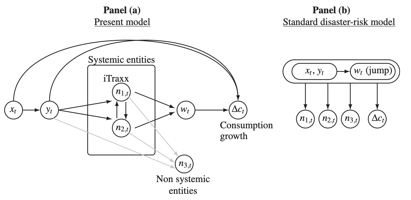
Figure 7.8: Causality scheme in Gourieroux et al. (2021).

In this context, a wide range of credit derivatives can be priced. In particular those whose payoffs depend on the default status of the constituents of a reference portfolio: Credit Index swaps (CIS) and synthetic CDO.

• CDS: protection payoff \(>0\), when the entity on which the CDS is written defaults.
• CIS: protection payoff \(>0\), when one entity of the underlying portfolio defaults.
• CDO: protection payoff \(>0\), when one entity of the underlying portfolio defaults, given that losses are in a given interval \([a,b]\) (e.g. \([a,b]=[3\%,6\%]\)). See Figure 7.9.

Typical credit indices are the iTraxx (Europe) and CDX (U.S.); these indices track the default status of 125 large firms.

The pricing CDO formula make an intensive use of the truncated Laplace transform (see Eq. (1.18), Darrell Duffie, Pan, and Singleton (2000)). The model estimation would be infeasible without the tractability provided by affine processes.

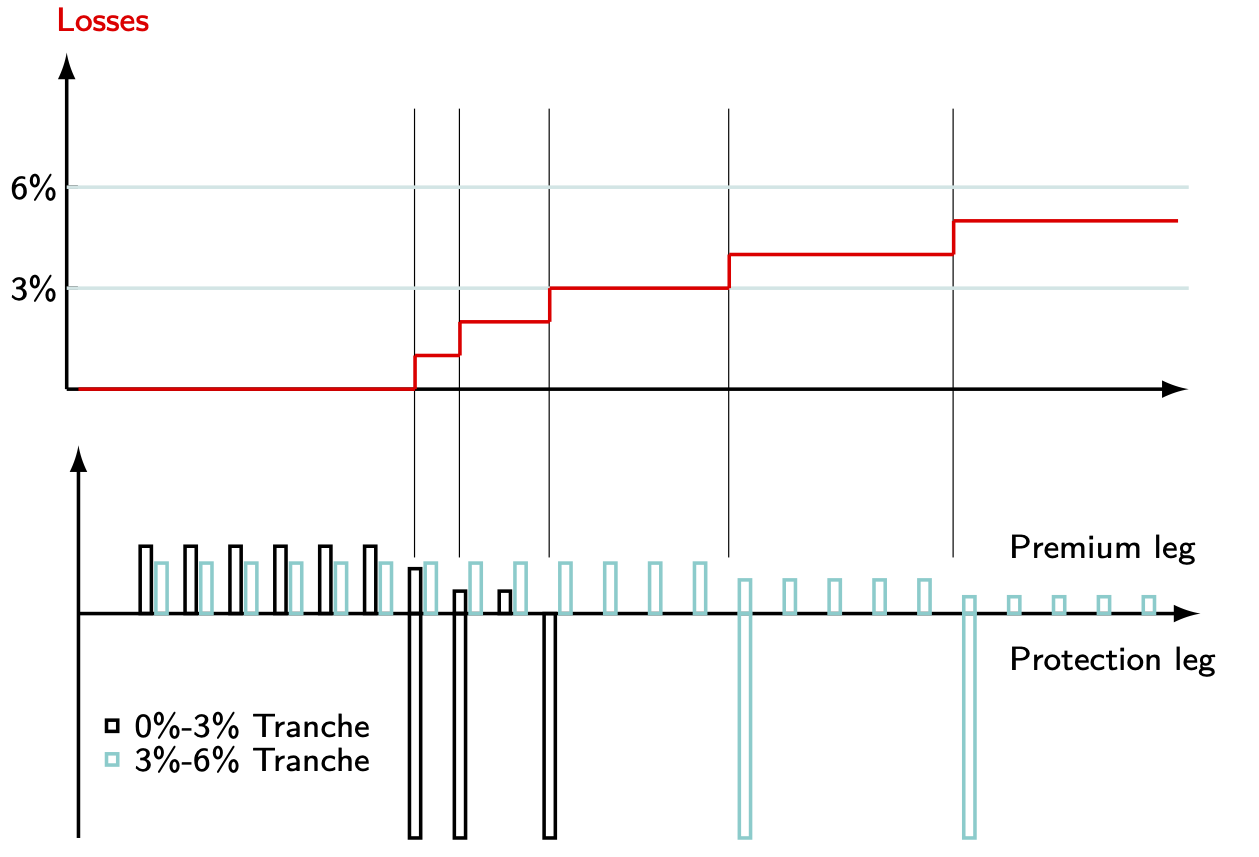
Figure 7.9: Collaterlized Debt Obligations (CDOs).

7.6 The shadow-intensity framework

7.6.1 Overview

Pallara and Renne (2023) and Renne and Pallara (2023) investigate the pricing the sovereign credit risk in the context of shadow-intensity frameworks. In that type of framework, the prices of defaultable bonds are given by conditional expectations of the form: \[\begin{equation} \mathbb{E}^{\mathbb{Q}}_t(\exp[\color{blue}{-z_{t+1}-\dots-z_{t+h}}-\max(0,\lambda_{t+1})-\dots -\max(0,\lambda_{t+h})]),\tag{7.41} \end{equation}\] where \(z_t\) (risk-free short-term rate) and \(\lambda_t\) (shadow default intensity) are affine functions of the state vector \(w_t\). In addition, \(y_t\) follows a Gaussian vector auto-regressive (VAR) model. That is, we have: \[\begin{eqnarray*} z_t &=& \dot{a}'y_t + \dot{b}\\ \lambda_t &=& a'y_t + b, \end{eqnarray*}\] and \[\begin{equation} y_t = \mu + \Phi y_{t-1}+ \Sigma\varepsilon_t,\tag{7.42} \end{equation}\] with \(\varepsilon_t \sim \mathcal{N}(0,Id)\) (where \(Id\) denotes the identity matrix).

Equation (7.41) gives the risk-neutral price of a bond of maturity \(h\), issued by an entity whose default intensity is \(\underline{\lambda}_t = \max(0,\lambda_t)\). (That is, the conditional default probability of the issuer, on date \(t\), is \(1-\exp(-\underline{\lambda}_t)\).) Because of the (nonlinear) max operator, the default intensity is not affine and the conditional expectation (7.41) cannot be computed using the standard affine-process machinery.

Absent the blue terms, the conditional expectations appearing in (7.41) would be of the same type as the ones considered in the shadow-rate literature (see Subsection 4.4.1). In that case, one could for instance use the approaches proposed by Priebsch (2013) or Wu and Xia (2016) to calculate approximations for these conditional expectations. Pallara and Renne (2023) and Renne and Pallara (2023) extend the approach of Wu and Xia (2016) to compute approximate values to (7.41). Th present page uses the latter approach, employing codes contained in package TSModels to implement this approach.

7.6.2 A numerical example

Consider a two-factor model, that is \(y_t = [y_{1,t},y_{2,t}]'\). Assume that \(z_t\) (that can be interpreted as the risk-free short term rate) depends on \(y_{1,t}\) only, and that \(\lambda_t\) (the shadow default intensity) depends on \(y_{2,t}\).

We consider the following VAR dynamics for \(y_t\): \[ y_t = \left[\begin{array}{cc}0.9 & 0 \\ 0 & 0.9\end{array}\right] y_{t-1} + \left[\begin{array}{cc}1 & 0.1 \\ 0 & 1\end{array}\right]\varepsilon_t, \] which determines \(\mu\), \(\Phi\), and \(\Sigma\) of (7.42).

Further, we want \(z_t\) (respectively \(\lambda_t\)) to be of mean 2% (respectively 0) and of standard deviation \(1\%\) (resp. 2/%).

Let us code these specifications:

Phi_x <- .9 * diag(2) # set Phi
Sigma_x <- diag(2) # set Sigma
Sigma_x[1,2] <- .1
Mu_x <- matrix(0,2,1) # set mu
stdv.z      <- .01 # set the unconditional std dev of z
stdv.lambda <- .02 # set the unconditional std dev of lambda
# Compute the unconditional variance of y_t:
uncond.Variance.X <- matrix(solve(diag(2*2) - Phi_x %x% Phi_x) %*%
                              c(Sigma_x %*% t(Sigma_x)),2,2)
# Deduce a and a.dot:
a.dot <- matrix(c(stdv.z/sqrt(uncond.Variance.X[1,1]),0))
a     <- matrix(c(0,stdv.lambda/sqrt(uncond.Variance.X[2,2])))
# Set the unconditional means of and lambda:
b.dot <- .02; b <- .0

Let us have a look at simulated paths for \(z_t\) and \(\lambda_t\):

library(TSModels)

nb.periods <- 200
X <- simul.X(Phi_x,Mu_x,Sigma_x,nb.periods)
z <- b.dot + a.dot[1] * X[1,1,]
lambda <- b + a[2] * X[2,1,]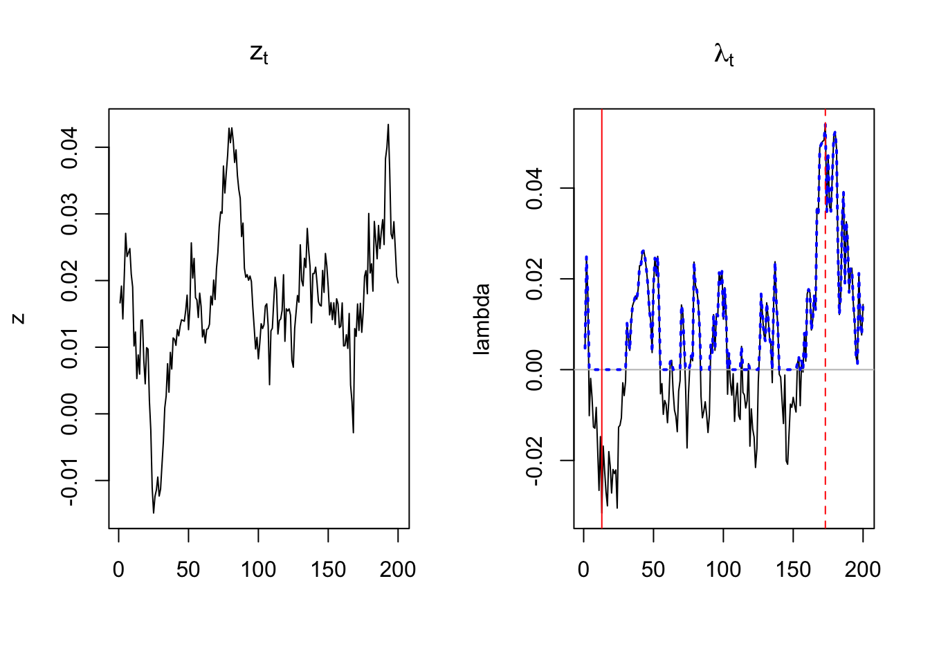

Figure 7.10: This plots shows simulated paths for \(z_t\) (risk-free short-term rate) and \(\lambda_t\) (shadow intensity). The blue dotted line, on the right-hand-side plot, is the effective intensity, that is \(\max(0,\lambda_t)\). The vertical lines indicate those dates where lambda is minimal and maximal.

7.6.3 Bond pricing

Let us now evaluate the conditional expectations of (7.41), for \(h=\{1,\dots,10\}\). For that, we make use of function compute.condit.Exp of package TSModels.

H <- 10
res <- compute.condit.Exp(a,b,a.dot,b.dot,
                          Phi_x,Mu_x,Sigma_x,
                          X=cbind(X[1,1,],X[2,1,]),
                          max.h = H)
t.min.lambda <- which(lambda==min(lambda))
t.max.lambda <- which(lambda==max(lambda))
rbind(res$E.n[t.max.lambda,], #approximate values of the conditional expect. for date t
      -log(res$E.n[t.max.lambda,])/(1:H))

##            [,1]       [,2]       [,3]       [,4]       [,5]       [,6]
## [1,] 0.93656698 0.88124243 0.83268158 0.78980533 0.75170565 0.71762216
## [2,] 0.06553424 0.06321126 0.06103466 0.05899219 0.05708209 0.05530201
##            [,7]       [,8]       [,9]      [,10]
## [1,] 0.68692286 0.65908502 0.63367728 0.61034360
## [2,] 0.05364761 0.05211284 0.05069061 0.04937332

The last two lines respectively give, for the date featuring the highest \(\lambda_t\), the term structures of the bond prices and of associated yields-to-maturity.

Let us now compute credit-risk-free bond prices. This is obtained by taking \(a=0\) and \(b=0\) (so that \(\lambda_t=0\)):

res0 <- compute.condit.Exp(a*0.00001,b*0.00001,a.dot,b.dot,
                          Phi_x,Mu_x,Sigma_x,
                          X=cbind(X[1,1,],X[2,1,]),
                          max.h = H)
y       <- - log(res$E.n) / t(matrix(1:H,H,nb.periods))
y_RF    <- - log(res0$E.n) / t(matrix(1:H,H,nb.periods))
spreads <- y - y_RF

Let us plot the term structures of yields and spreads for the date on which we observe the highest \(\lambda_t\):

plot(y[t.max.lambda,],type="l",ylim=c(0,max(y)),xlab="maturity",ylab="yields",
     main="Term structures of bond yields (risk-free and defaultable bonds)",lwd=2)
lines(y_RF[t.max.lambda,],col="red",lwd=2)
lines(y_RF[t.min.lambda,],col="red",lwd=2,lty=2)
lines(y[t.min.lambda,],lwd=2,lty=2)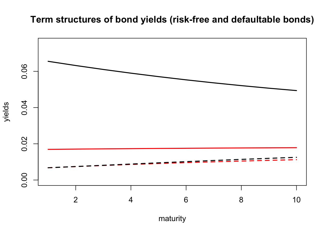

Figure 7.11: Term structures of risk-free yields (in red), and credit-risky yields (in black). Solid lines (respectively dashed lines) correspond to the date where \(\lambda_t\) is the highest (resp. the lowest). These two dates are indicated by vertical lines on the previous figure.

Let us check the formulas by simulations. More precisely, we calculate the conditional expectation given in (7.41) using Monte-Carlo simulations, for different maturities \(h\). We will then compare these prices with the ones resulting from function compute.condit.Exp. We consider the date on which \(\lambda_t\) is the highest.

nb.replics <- 10000 # Number of simulated trajectories
t  <- t.max.lambda # date on which cond. expect. are computed
Xt <- matrix(X[,1,t],ncol=1) # state vector on that date

# Simulate trajectories starting from Xt:
X <- simul.X(Phi_x,Mu_x,Sigma_x,nb.periods=H,X0 = Xt,
             nb.replics = nb.replics)
# Compute prices for each trajectory:
aux1 <- apply(X,c(2,3),function(x){exp(- b.dot - t(x)%*%a.dot -
                                        pmax(0,b + t(x)%*%a))})
aux2 <- apply(aux1,1,cumprod)
# Compute averages of prices across simulated trajectories:
simul.prices <- apply(aux2,1,mean)
# Compare with output of compute.condit.Exp:
plot(res$E.n[t,],lwd=2,
     main="Approximate formula versus Monte-Carlo approach")
lines(simul.prices)
legend("topright",c("Approximate formula","Monte-Carlo"),
       lty=c(NaN,1),pch=c(1,NaN),lwd=c(2,1))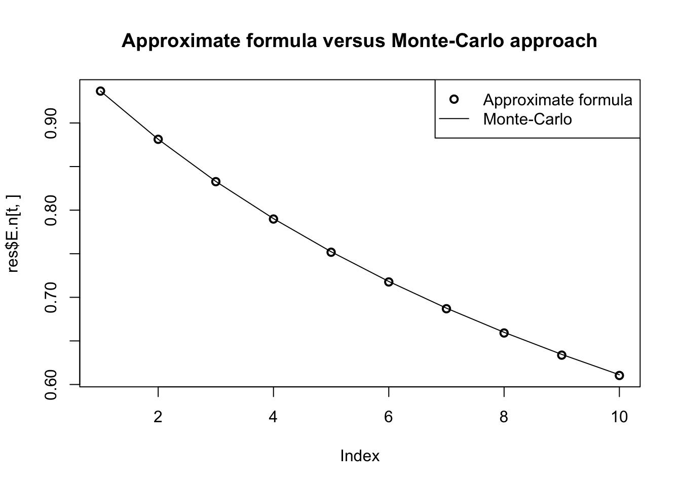

Figure 7.12: Comparison between formula-based prices and Monte-Carlo-based defaultable bond prices.