7 ARCH and GARCH models

7.1 Conditional heteroskedasticity

Many financial and macroeconomic variables are hit by shocks whose variance is not constant through time, i.e. by heteroskedatic shocks. Often, the conditional variance of shocks features a persistent behavior (volatility clustering). The observation that large shocks (in absolute value) tend to be followed by other important shocks has notably been established by Mandelbrot (1963). Such a situation is illustrated by Figure 7.1.

Autoregressive Conditional Heteroskedasticity (ARCH) and its generalized version (GARCH) constitute useful tools to model such time series.

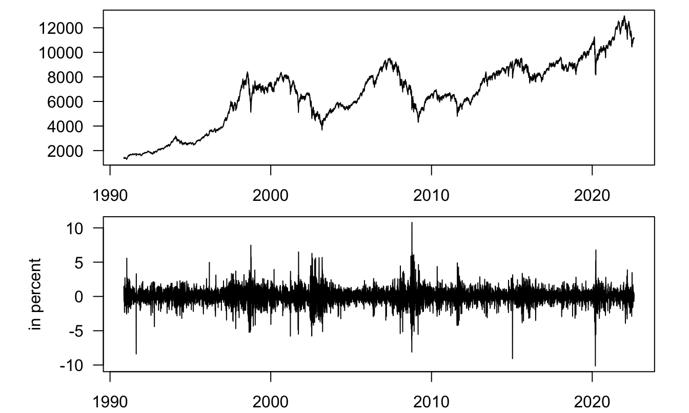
Figure 7.1: Upper plot: SMI index (daily Close prices); lower plot: daily log returns.

In order to test whether a times series of shocks \(\{u_1,\dots,u_T\}\) features persistent conditional heteroskedasticity, a simple test has been designed by Engle (1982). This test consists in regressing \(u_t^2\) on it last \(m\) lags (i.e., on \(u_{t-1}^2,\dots,u_{t-m}^2\)) by OLS.Under the null hypothesis that \(u_t\) is i.i.d., we have: \[ T \times R^2 \overset{d}{\rightarrow} \chi^2(m), \] where \(R^2\) is the centered \(R^2\) of the OLS regression.

Let us employ this test on the return series plotted in the lower panel of Figure 7.1:

library(AEC);data(smi)
smi <- smi[complete.cases(smi),] # remove NaNs
T <- dim(smi)[1]
smi$r <- 100*c(NaN,log(smi$Close[2:T]/smi$Close[1:(T-1)]))
u <- smi$r^2
u_1 <- c(NaN,smi$r[1:(T-1)]^2)
u_2 <- c(NaN,NaN,smi$r[1:(T-2)]^2)
eq <- lm(u^2 ~ u_1^2 + u_2^2)
test.stat <- length(u)*summary(eq)$r.squared
pvalue <- 1 - pchisq(q = test.stat,df=2)

The p-value is extremely close to zero. Hence we strongly reject the null of an i.i.d. SMI return.

7.2 The ARCH model

7.2.1 The two ARCH specifications

Consider the auto-regressive process following: \[\begin{equation} y_t = c + \phi_1 y_{t-1} + \dots + \phi_p y_{t-p} + u_t,\tag{7.1} \end{equation}\] where \(u_t\) is a white noise (Def. 1.1), i.e. \(\mathbb{E}(u_t)=0\), \(\mathbb{E}(u_t^2)=\sigma^2\) and \(\mathbb{E}(u_t u_s)=0\) if \(s \ne t\). Importantly, note that while the unconditional variance of \(u_t\) is \(\sigma^2\), its conditional variance can be time-varying. This is the case in the context of (G)ARCH models.

In the ARCH(m) model, \(u_t\) follows: \[\begin{equation} u_t^2 = \zeta + \alpha_1 u_{t-1}^2 + \dots + \alpha_m u_{t-m}^2 + w_t,\tag{7.2} \end{equation}\] where \(w_t\) is a non-autocorrelated white noise process that is exogenous to \(u_t\), in the sense that: \[ \mathbb{E}(w_t|u_{t-1},u_{t-2},\dots)=0. \] In this case: \[\begin{equation} \mathbb{E}(u_t^2|u_{t-1},u_{t-2},\dots) = \zeta + \alpha_1 u_{t-1}^2 + \dots + \alpha_m u_{t-m}^2.\tag{7.3} \end{equation}\]

For Eq. (7.2) to make sense, it has to be the case that \[ \zeta + \alpha_1 u_{t-1}^2 + \dots + \alpha_m u_{t-m}^2 + w_t \ge 0 \] for all realisations of \(\{u_t\}\). This is the case if \(w_t > -\zeta\), with \(\zeta>0\), and if \(\alpha_i \ge 0\) for \(i \in \{1,\dots,m\}\). Assuming this is the case, \(u_t^2\) is covariance-stationary if the roots of: \[ g(z) = 1 - \alpha_1 z - \dots - \alpha_m z^m = 0 \] lie outside the unit circle (Prop. 2.5). A necessary condition for not having a root between 0 and 1 is that \(\sum_i \alpha_i<1\).¹⁸ This is also a sufficient condition.¹⁹

If \(w_t > -\zeta\), with \(\zeta>0\), \(\alpha_i\ge0\) for \(i \in \{1,\dots,m\}\) and \(\sum_i \alpha_i<1\), then the unconditional variance of \(u_t\) is: \[ \sigma^2 = \mathbb{E}(u_t^2) = \frac{\zeta}{1 - \sum_{i=1}^m \alpha_i}. \]

An alternative representation of an ARCH(m) process is as follows: \[\begin{equation} u_t = \sqrt{h_t}v_t,\tag{7.4} \end{equation}\] where \(v_t\) is an i.i.d. sequence with zero mean and unit variance, i.e.: \[ \mathbb{E}(v_t) = 0, \quad \mathbb{E}(v_t^2) = 1. \] If \(h_t\) follows: \[\begin{equation} h_t = \zeta + \alpha_1 u_{t-1}^2 + \dots + \alpha_m u_{t-m}^2,\tag{7.5} \end{equation}\] then Eq. (7.3) is also true. Since \(u_t^2 = h_t v_t^2\), Eq. (7.2) holds with \(w_t = h_t (v_t^2-1)\). This alternative representation is convenient because \(v_t\) is not necessarily bounded.

7.2.2 Maximum Likelihood Estimation of an ARCH process

Assume the complete model is: \[ y_t = \mathbf{x}_t'\boldsymbol\beta + u_t, \] where \(\mathbf{x}_t\) is a \(k \times 1\) vector of explanatory variables and \(u_t\) is as specified in Eq. (7.4).

To write the likelihood function, it is convenient to condition on the first \(m\) observations. Let us denote by \(\mathcal{I}_t\) the following information set: \[ \mathcal{I}_t = (y_t,y_{t-1},\dots,y_0,y_{-1},\dots,y_{-m+1}, \mathbf{x}_t,\mathbf{x}_{t-1},\dots,\mathbf{x}_0,\mathbf{x}_{-1},\dots,\mathbf{x}_{-m+1}). \]

If \(v_t \sim \mathcal{N}(0,1)\), we have, for \(t\ge1\): \[\begin{equation} f(y_t|\mathbf{x_t},\mathcal{I}_{t-1}) = \frac{1}{\sqrt{2 \pi h_t}}\exp\left(\frac{-(y_t-\mathbf{x}_t'\boldsymbol\beta)^2}{2h_t}\right),\tag{7.6} \end{equation}\] where \(h_t\) is given by: \[ h_t = \zeta + \alpha_1 (y_{t-1} - \mathbf{x}_{t-1}'\boldsymbol\beta)^2 + \dots + \alpha_m (y_{t-m} - \mathbf{x}_{t-m}'\boldsymbol\beta)^2. \]

The log likelihood function is given by: \[ \log \mathcal{L}(\theta) = \sum_{t=1}^T \log(f(y_t|\mathbf{x_t},\mathcal{I}_{t-1})), \] where \(\theta\), the vector of unknown parameters, is \([\boldsymbol\beta',\zeta,\boldsymbol\alpha']'\), where \(\boldsymbol\alpha=[\alpha_1,\dots,\alpha_m]'\). The maximisation of the log likelihood is performed numerically.

Note that one can also use non-Gaussian distributions for \(v_t\). (For that, one has to replace the normal distribution in Eq. (7.6).)

Let us fit an ARCH(2) model on the SMI return data (lower plot of Figure 7.1). For this, we make use of function compute.garch of package AEC. This function takes four arguments:

• vector theta contains the model parameterization: first, \(\zeta\), then the \(\alpha_i\)’s, then for GARCH models (see Subsection 7.3 below), the \(\delta_i\)’s.
• vector x contains the observations of the process.
• m is the number of lags in the ARCH specification.
• r is the number of lags in the GARCH specification (see Subsection 7.3 below).

Function compute.garch returns a list, one entry of each is the log-likelihood associated with a parameterization \([\zeta,\boldsymbol\alpha']'\), the second being the resulting sequence of \(h_t\)’s (see Eq. (7.5)). Let us create a function that returns only the log-likelihood:

loglik <- function(theta,x,m,r){
  # first parameter of theta: zeta
  # next: alpha's (ARCH)
  # next: delta's (GARCH)
  Garch <- compute.garch(theta,x,m,r)
  return(Garch$logf)
}

Now, let us maximize the log-likelihood:

m <- 2
r <- 0 # for ARCH models, r=0
smi <- smi[4000:dim(smi)[1],] # reduce sample
par0 <- c(0.62,0.2,0.2)
res.opt <- optim(par=par0,x=smi$r,m=m,r=r,loglik,
                 method="BFGS",hessian=TRUE,
                 control = list(trace=TRUE,maxit = 10))
estim.param <- res.opt$par
std.dev <- sqrt(diag(solve(res.opt$hessian)))
t.stat <- estim.param/std.dev

Table 7.1 reports the estimated parameters and their standard deviation. Figure 7.2 displays the resulting 95% confidence intervals (i.e., \(\pm 2 \sqrt{h_t}\)).

Table 7.1: ARCH(2), ML estimation results. Data: SMI daily returns.

	Estim. param.	Std dev.	t-stat
zeta	0.6042	0.0230	26.3054
alpha1	0.2939	0.0289	10.1704
alpha2	0.2321	0.0250	9.2838

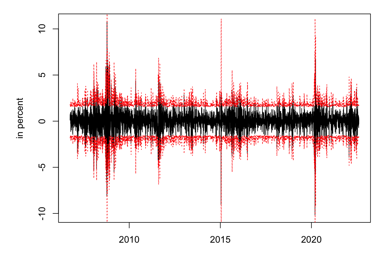
Figure 7.2: SMI daily returns (in black) and, in red, 95% confidence interval based on the ARCH(2) estimated model (\(\pm 2 \sqrt{h_t}\)).

7.3 The GARCH model

One can generalize the model and replace Eq. (7.5) with: \[\begin{eqnarray} h_t &=& (1-\delta_1 - \delta_2 - \dots - \delta_r) \zeta + \nonumber \\ &&\delta_1 h_{t-1} + \delta_2 h_{t-2} + \dots + \delta_r h_{t-r} + \nonumber \\ &&\alpha_1 u_{t-1}^2 + \dots + \alpha_m u_{t-m}^2. \tag{7.7} \end{eqnarray}\] This generalised autoregressive conditional heteroskedasticity model is denoted by GARCH(r,m). Non-negativity is satisfied as soon as \(\kappa>0\), \(\alpha_j \ge 0\), \(\delta_j \ge 0\) for \(j \le p\).

Denoting \(u_t^2 - h_t\) by \(w_t\), and \((1-\delta_1 - \dots - \delta_r) \zeta\) by \(\kappa\), it can be checked that:²⁰ \[\begin{eqnarray} u_t^2 &=& \kappa + (\delta_1 + \alpha_1)u_{t-1}^2 + (\delta_2 + \alpha_2)u_{t-2}^2 + \dots \nonumber \\ && + (\delta_p + \alpha_p)u_{t-p}^2 + w_t - \delta_1 w_{t-1} - \dots - \delta_r w_{t-r}, \end{eqnarray}\] where \(p=max(m,r)\), \(\alpha_j=0\) for \(j>m\) and \(\delta_j=0\) for \(j>r\).

We have \(w_t = h_t(v_t^2 - 1)\). Under regularity assumptions, \(\{w_t\}\) is a white noise. Hence, \(u_t^2\) follows an ARMA(p,r) process. Accordingly, it comes that \(u_t^2\) is covariance stationary if the roots of: \[ 1 - (\delta_1 + \alpha_1)z - \dots - (\delta_1 + \alpha_1)z^p = 0 \] lie outside the unit circle (Prop. 2.5). When the \(\delta_i + \alpha_i\) are nonnegative, and using the same reasoning as for ARCH models, this is the case iff: \[ \sum_i \delta_i + \sum_i \alpha_i < 1. \] In that case, the unconditional variance of \(u_t\), i.e. the unconditional mean of \(u_t^2\), is: \[ \mathbb{E}(u_t^2) = \sigma^2 = \frac{\kappa}{1 - \sum_i \delta_i - \sum_i \alpha_i}. \]

GARCH models can also be estimated by the ML approach.Table 7.2 reports the estimated parameters when fitting an GARCH(1,1) model on the SMI return dataset. Figure

Figure 7.3 compare the condiitonal standard deviations (\(\sqrt{h_t}\)) resulting from the ARCH(2) and the GARCH(1,1) specifications.

## initial  value 5703.217726 
## iter  10 value 5359.604659
## final  value 5359.604659 
## stopped after 10 iterations

Table 7.2: ARCH(2), ML estimation results. Data: SMI daily returns.

	Estim. param.	Std dev.	t-stat
zeta	0.2195	0.0216	10.1753
alpha1	0.1450	0.0152	9.5297
delta1	0.8299	0.0152	54.5175

Figure 7.3: Estimated conditional standard deviations (\(\sqrt{h_t}\)) of SMI daily returns: ARCH(2) [black line] and GARCH(1,1) [dotted red line] specifications.

7.4 ARCH-in-mean

Another extension of the ARCH model is the ARCH-in-Mean, or ARCH-M model. That model is close to that specified by Eqs. (7.1), (7.4) and (7.5), but it also allows for a potential effect of \(h_t\) on \(\mathbb{E}_{t-1}(y_{t})\): \[\begin{eqnarray*} y_t &=& c + \phi_1 y_{t-1} + \dots + \phi_p y_{t-p} + {\color{blue}\delta h_t}+ u_t \\ u_t &=& \sqrt{h_t} v_t \\ h_t &=& \zeta + \alpha_1 u_{t-1}^2 + \dots + \alpha_m u_{t-m}^2, \end{eqnarray*}\] where \(v_t\) is a zero-mean unit-variance i.i.d. sequence.