1 Basics

1.1 Shocks and lag operator

A time series is an infinite sequence of random variables indexed by time: $\{y_t\}_{t=-\infty}^{+\infty}=\{\dots, y_{-2},y_{-1},y_{0},y_{1},\dots,y_t,\dots\}$, $y_i \in \mathbb{R}^k$. In practice, we only observe samples, typically: $\{y_{1},\dots,y_T\}$.

Standard time series models are built using shocks that we will often denote by $\varepsilon_t$. Typically, $\mathbb{E}(\varepsilon_t)=0$. In many models, the shocks are supposed to be i.i.d., but there exist other (less restrictive) notions of shocks. In particular, the definition of many processes is based on white noises:

Definition 1.1 (White noise) The process $\{\varepsilon_t\}_{t \in] -\infty,+\infty[}$ is a white noise if, for all $t$:

$\mathbb{E}(\varepsilon_t)=0$,
$\mathbb{E}(\varepsilon_t^2)=\sigma^2<\infty$,
for all $s\ne t$, $\mathbb{E}(\varepsilon_t \varepsilon_s)=0$.

Another type of shocks that are commonly used are Martingale Difference Sequences:

Definition 1.2 (Martingale Difference Sequence) The process $\{\varepsilon_t\}_{t = -\infty}^{+\infty}$ is a martingale difference sequence (MDS) if $\mathbb{E}(|\varepsilon_{t}|)<\infty$ and if, for all $t$, \[ \underbrace{\mathbb{E}_{t-1}(\varepsilon_{t})}_{\mbox{conditional on the past}}=0. \]

By definition, if $y_t$ is a martingale, then $y_{t}-y_{t-1}$ is a MDS.

Example 1.1 (ARCH process) The Autoregressive conditional heteroskedasticity process—studied in Section 7—is an example of shock that satisfies the white noise and MDS definitions, but that is not i.i.d.: \[ \varepsilon_{t} = \sigma_t \times z_{t}, \] where $z_t \sim i.i.d.\,\mathcal{N}(0,1)$ and $\sigma_t^2 = w + \alpha \varepsilon_{t-1}^2$ (with $w>0$ and $0 \leq \alpha <1$).

T <- 500
w <- 1; alpha <- .98
all_epsilon <- NULL; epsilon_1 <- 0
for(t in 1:T){
  sigma <- sqrt(w + alpha * epsilon_1^2)
  epsilon <- sigma * rnorm(1)
  all_epsilon <- c(all_epsilon,epsilon)
  epsilon_1 <- epsilon
}
par(plt=c(.15,.95,.1,.95))
plot(all_epsilon,type="l",lwd=2,
     ylab=expression(epsilon[t]),xlab="")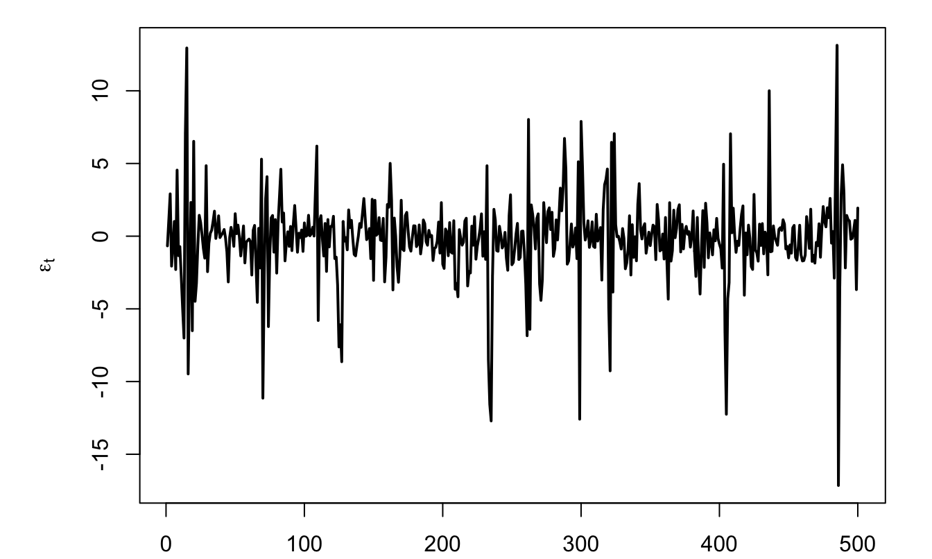

$Simulation of $\varepsilon_t$, where $\varepsilon_{t} = \sigma_t \times z_{t}$, with $z_t \sim i.i.d.\,\mathcal{N}(0,1)$.$

Figure 1.1: Simulation of $\varepsilon_t$, where $\varepsilon_{t} = \sigma_t \times z_{t}$, with $z_t \sim i.i.d.\,\mathcal{N}(0,1)$.

Example 1.2 A white noise process is not necessarily a MDS. This is for instance the case for following process: \[ \varepsilon_{t} = z_t + z_{t-1}z_{t-2}, \] where $z_t \sim i.i.d.\mathcal{N}(0,1)$.

Indeed, it can be shown that the $\varepsilon_t$’s are not correlated through time, we have $\mathbb{E}_{t-1}(\varepsilon_t)=z_{t-1}z_{t-2} \ne 0$.

In the following, to simplify the exposition, we will essentially consider strong white noises. A strong white noise is a particular case of white noise where the $\varepsilon_{t}$’s are serially independent. Using the law of iterated expectation, it can be shown that a strong white noise is a martingale difference sequence. Indeed, when the $\varepsilon_{t}$’s are serially independent, we have that $\mathbb{E}(\varepsilon_{t}|\varepsilon_{t-1},\varepsilon_{t-2},\dots)=\mathbb{E}(\varepsilon_{t})=0$, as $f_{\mathcal{E}_t}(\varepsilon_t|\varepsilon_{t-1},\varepsilon_{t-2},\dots)=f_{\mathcal{E}_t}(\varepsilon_t)$.

Let us now introduce the lag operator. The lag operator, denoted by $L$, is defined on the time series space and is defined by: \[\begin{equation} L: \{y_t\}_{t=-\infty}^{+\infty} \rightarrow \{w_t\}_{t=-\infty}^{+\infty} \quad \mbox{with} \quad w_t = y_{t-1}.\tag{1.1} \end{equation}\]

It is easily seen that we have $L^2 y_t =L(L y_t) = y_{t-2}$ and, more generally, $L^k y_t = y_{t-k}$.

Consider a process $y_t$ whose law of motion is $y_t = \mu + \phi y_{t-1} + \varepsilon_t$, where the $\varepsilon_t$’s are i.i.d. $\mathcal{N}(0,\sigma^2)$ (this is an AR(1) process, as we will see in Section 2). Using the lag operator, the dynamics of $y_t$ can be expressed as follows: \[ (1-\phi L) y_t = \mu + \varepsilon_t. \]

1.2 Conditional and unconditional moments

If it exists, the unconditional (or marginal) mean of the random variable $y_t$ is given by: \[ \mu_t := \mathbb{E}(y_t) = \int_{-\infty}^{\infty} y_t f_{Y_t}(y_t) dy_t, \] where $f_{Y_t}$ is the unconditional, or marginal, density (p.d.f.) of $y_t$. Note that, in the general case, $Y_t$ and $Y_{t-1}$, may have different densities; that is, in general, $f_{Y_t} \ne f_{Y_{t-1}}$ (and, in particular, $\mu_t \ne \mu_{t-1}$).

Similarly, if it exists, the unconditional (or marginal) variance of the random variable $y_t$ is: \[ \mathbb{V}ar(y_t) = \int_{-\infty}^{\infty} (y_t - \mathbb{E}(y_t))^2 f_{Y_t}(y_t) dy_t. \]

Definition 1.3 (Autocovariance) The $j^{th}$ autocovariance of $y_t$ is given by: \[\begin{eqnarray*} \gamma_{j,t} &:=& \mathbb{E}([y_t - \mathbb{E}(y_t)][y_{t-j} - \mathbb{E}(y_{t-j})])\\ &=& \int_{-\infty}^{\infty} \int_{-\infty}^{\infty} \dots \int_{-\infty}^{\infty} [y_t - \mathbb{E}(y_t)][y_{t-j} - \mathbb{E}(y_{t-j})] \times\\ && f_{Y_t,Y_{t-1},\dots,Y_{t-j}}(y_t,y_{t-1},\dots,y_{t-j}) dy_t dy_{t-1} \dots dy_{t-j}, \end{eqnarray*}\] where $f_{Y_t,Y_{t-1},\dots,Y_{t-j}}(y_t,y_{t-1},\dots,y_{t-j})$ is the joint distribution of $y_t,y_{t-1},\dots,y_{t-j}$.

In particular, note that $\gamma_{0,t} = \mathbb{V}ar(y_t)$.

Definition 1.4 (Covariance stationarity) The process $y_t$ is covariance stationary —or weakly stationary— if, for all $t$ and $j$, \[ \mathbb{E}(y_t) = \mu \quad \mbox{and} \quad \mathbb{E}\{(y_t - \mu)(y_{t-j} - \mu)\} = \gamma_j. \]

Figure 1.2 displays the simulation of a process that is not covariance stationary. This process follows $y_t = 0.1t + \varepsilon_t$, where $\varepsilon_t \sim\,i.i.d.\,\mathcal{N}(0,1)$. Indeed, for such a process, we have: $\mathbb{E}(y_t)=0.1t$, which depends on $t$.

T <- 200
y <- 0.1*(1:T) + rnorm(T)
par(plt=c(.1,.95,.1,.95))
plot(y,xlab="",ylab="",lwd=2,type="l")

$Example of a process that is not covariance stationary. it follows: $y_t = 0.1t + \varepsilon_t$, where $\varepsilon_t \sim \mathcal{N}(0,1)$.$

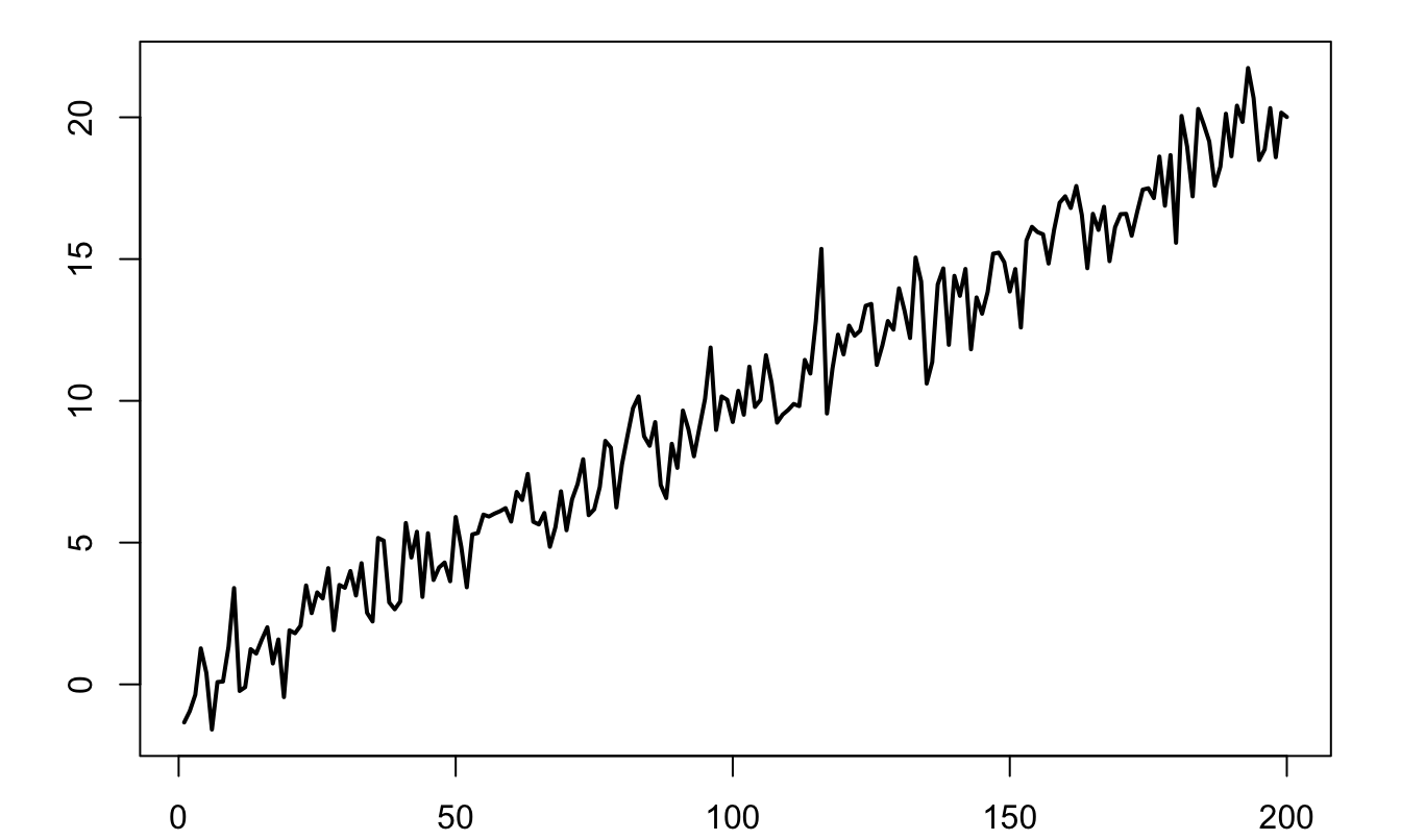
Figure 1.2: Example of a process that is not covariance stationary. it follows: $y_t = 0.1t + \varepsilon_t$, where $\varepsilon_t \sim \mathcal{N}(0,1)$.

Definition 1.5 (Strict stationarity) The process $y_t$ is strictly stationary if, for all $t$ and all sets of integers $J=\{j_1,\dots,j_n\}$, the distribution of $(y_{t},y_{t+j_1},\dots,y_{t+j_n})$ depends on $J$ but not on $t$.

The following process is covariance stationary but not strictly stationary: \[ y_t = \mathbb{I}_{\{t<1000\}}\varepsilon_{1,t}+\mathbb{I}_{\{t\ge1000\}}\varepsilon_{2,t}, \] where $\varepsilon_{1,t} \sim \mathcal{N}(0,1)$ and $\varepsilon_{2,t} \sim \sqrt{\frac{\nu - 2}{\nu}} t(\nu)$ and $\nu = 4$¹. A simulated path is displayed in Figure 1.3.

T <- 2000
y <- rnorm(T)
y[(T/2):T] <- rt(n = T/2 + 1,df=4)
par(plt=c(.1,.95,.15,.95))
plot(y,xlab="",ylab="",type="l")
abline(h=-2.58,col="red",lty=3)
abline(h=2.58,col="red",lty=3)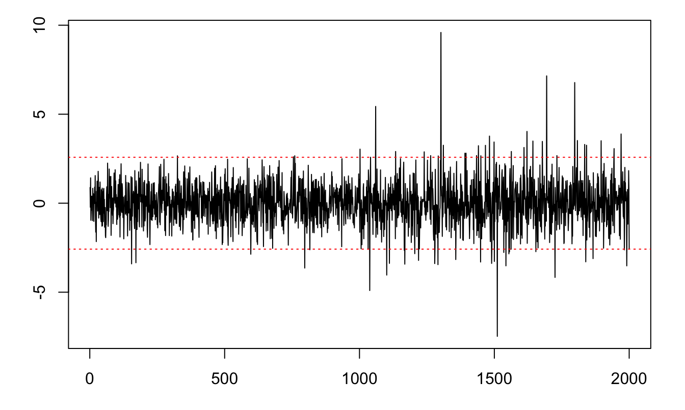

$Example of a process that is covariance stationary but not strictly stationary. The red lines delineate the 99\% confidence interval of the standard normal distribution ($\pm 2.58$).$

Figure 1.3: Example of a process that is covariance stationary but not strictly stationary. The red lines delineate the 99% confidence interval of the standard normal distribution ($\pm 2.58$).

Proposition 1.1 If $y_t$ is covariance stationary, then $\gamma_j = \gamma_{-j}$.

Proof. Since $y_t$ is covariance stationary, the covariance between $y_t$ and $y_{t-j}$ (i.e., $\gamma_j$) is the same as that between $y_{t+j}$ and $y_{t+j-j}$ (i.e. $\gamma_{-j}$).

Definition 1.6 (Auto-correlation) The $j^{th}$ auto-correlation of a covariance-stationary process is: \[ \rho_j = \frac{\gamma_j}{\gamma_0}. \]

Consider a long historical time series of the Swiss GDP growth, taken from the Jordà, Schularick, and Taylor (2017) dataset.²

library(AEC)
data(JST);data <- subset(JST,iso=="CHE")
par(plt=c(.1,.95,.1,.95))
T <- dim(data)[1]
data$growth <- c(NaN,log(data$gdp[2:T]/data$gdp[1:(T-1)]))
plot(data$year,data$growth,type="l",xlab="",ylab="",lwd=2)
abline(h=mean(data$growth,na.rm = TRUE),col="blue",lty=2,xlab="",ylab="")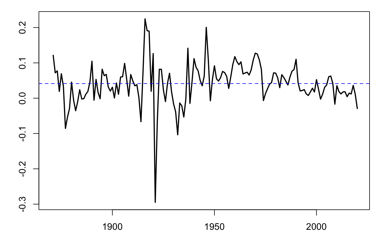

Figure 1.4: Annual growth rate of Swiss GDP, based on the Jorda-Schularick-Taylor Macrohistory Database.

Figure 1.5 shows two scatter plots. In the first one, the coordinates of each point are of the form $(y_{t-1},y_t)$. Hence, the slope of the OLS regression line (in blue) is $\widehat{\mathbb{C}ov}(y_t,y_{t-1})/\widehat{\mathbb{V}ar}(y_{t-1})$ (where the hats indicate that these moments are the sample ones). Assuming that the process is covariance stationary, the slope therefore is an estimate of the auto-correlation of order one. By the same logic, the slope of the blue line in the second plot is an estimate of the auto-correlation of order three.

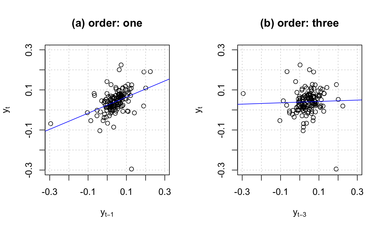
$For order $j$, the slope of the blue line is, approximately, $\hat{\gamma}_j/\widehat{\mathbb{V}ar}(y_t)$, where hats indicate sample moments.$

Figure 1.5: For order $j$, the slope of the blue line is, approximately, $\hat{\gamma}_j/\widehat{\mathbb{V}ar}(y_t)$, where hats indicate sample moments.

1.3 Central Limit Theorem (CLT) for persistent processes

This subsection shows that the Central Limit Theorem (CLT, see Theorem 8.5) can be extended to cases where the observations are auto-correlated.

Theorem 1.1 (Central Limit Theorem for covariance-stationary processes) If process $y_t$ is covariance stationary and if the series of autocovariances is absolutely summable ($\sum_{j=-\infty}^{+\infty} |\gamma_j| <\infty$), then: \[\begin{eqnarray} \bar{y}_T \overset{m.s.}{\rightarrow} \mu &=& \mathbb{E}(y_t) \tag{1.2}\\ \mbox{lim}_{T \rightarrow +\infty} T \mathbb{E}\left[(\bar{y}_T - \mu)^2\right] &=& \sum_{j=-\infty}^{+\infty} \gamma_j \tag{1.3}\\ \sqrt{T}(\bar{y}_T - \mu) &\overset{d}{\rightarrow}& \mathcal{N}\left(0,\sum_{j=-\infty}^{+\infty} \gamma_j \right) \tag{1.4}. \end{eqnarray}\]

[Mean square (m.s.) and distribution (d.) convergences: see Definitions 8.16 and 8.14.]

Proof. The absolute value of the series of the autocovariances is finite as it is lower than the sum of the absolute values of the autocovariances which is finite by the absolute summability assumption. As a result, there exists a finite $M \in \mathbb{R}$ such that $\sum_{j=-\infty}^{+\infty} \gamma_j=M$ and Eq. (1.3) implies Eq. (1.2). For Eq. (1.3), see Appendix 8.4. For Eq. (1.4), see Anderson (1971), p. 429.

Definition 1.7 (Long-run variance) Under the assumptions of Theorem 1.1, the limit appearing in Eq. (1.3) exists and is called long-run variance. It is denoted by $S$, i.e.: \[ S = \Sigma_{j=-\infty}^{+\infty} \gamma_j = \mbox{lim}_{T \rightarrow +\infty} T \mathbb{E}[(\bar{y}_T - \mu)^2]. \]

If $y_t$ is ergodic for second moments (see Def. 8.8), a natural estimator of $S$ is: \[\begin{equation} \hat\gamma_0 + 2 \sum_{\nu=1}^{q} \hat\gamma_\nu, \tag{1.5} \end{equation}\] where $\hat\gamma_\nu = \frac{1}{T}\sum_{\nu+1}^{T} (y_t - \bar{y})(y_{t-\nu} - \bar{y})$.

However, for small samples, Eq. (1.5) does not necessarily result in a positive definite matrix. Newey and West (1987) have proposed an estimator that does not have this defect. Their estimator is given by: \[\begin{equation} S^{NW}=\hat\gamma_0 + 2 \sum_{\nu=1}^{q}\left(1-\frac{\nu}{q+1}\right) \hat\gamma_\nu.\tag{1.6} \end{equation}\]

Loosely speaking, Theorem 1.1 says that, for a given sample size, the higher the “persistency” of a process, the lower the accuracy of the sample mean as an estimate of the population mean. To illustrate, consider three processes that feature the same marginal variance (equal to one, say), but different autocorrelations: 0%, 70%, and 99.9%. Figure 1.6 displays simulated paths of such three processes. It indeed appears that, the larger the autocorrelation of the process, the further the sample mean (dashed red line) from the population mean (red solid line).

The same type of simulations can be performed using this web interface (use panel “AR(1)”).

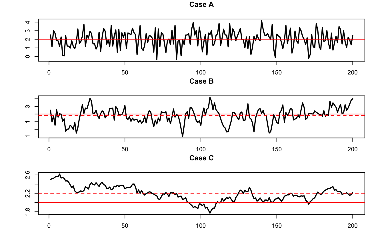
$The three samples have been simulated using the following data generating process: $x_t = \mu + \rho (x_{t-1}-\mu) + \sqrt{1-\rho^2}\varepsilon_t$, where $\varepsilon_t \sim \mathcal{N}(0,1)$. Case A: $\rho = 0$; Case B: $\rho = 0.7$; Case C: $\rho = 0.999$. In the three cases, $\mathbb{E}(x_t)=\mu=2$ and $\mathbb{V}ar(x_t)=1$. The dashed (respectively solid) red line indicate the sample (resp. unconditional) mean.$

Figure 1.6: The three samples have been simulated using the following data generating process: $x_t = \mu + \rho (x_{t-1}-\mu) + \sqrt{1-\rho^2}\varepsilon_t$, where $\varepsilon_t \sim \mathcal{N}(0,1)$. Case A: $\rho = 0$; Case B: $\rho = 0.7$; Case C: $\rho = 0.999$. In the three cases, $\mathbb{E}(x_t)=\mu=2$ and $\mathbb{V}ar(x_t)=1$. The dashed (respectively solid) red line indicate the sample (resp. unconditional) mean.

Introduction to Time Series

2 Univariate processes