Chapter 1 Basic statistical results

Econometrics describes populations, compares groups, and learns about unknown quantities from samples. This chapter introduces the probability tools used for those tasks. We begin with discrete random variables, for which joint and conditional distributions can be read directly from a table. Continuous distributions are introduced afterwards as the corresponding integral-based formulation.

Prerequisites. Basic probability, differentiation, and integration.

After working through this chapter, you should be able to:

• Calculate moments of a random variable and interpret variance and covariance.
• Move between joint, marginal, and conditional distributions.
• Use densities and distribution functions to calculate probabilities.
• Apply iterated expectations and decompose variance into within-group and between-group components.
• Distinguish bias, variance, mean squared error, and consistency.

Roadmap. We start with moments and discrete joint distributions, then move to continuous distributions. The laws of iterated expectations and total variance connect conditional and unconditional quantities. The final section introduces the main criteria used to assess estimators. The exercises in Section 1.8 develop these skills through calculations, proofs, and statements to assess.

1.1 Random variables and moments

A random variable assigns a numerical value to each possible outcome of an experiment. Its distribution describes which values it can take and how likely they are. If a discrete random variable \(X\) takes values \(x_1,\ldots,x_m\), write \[ p_X(x_j)=\mathbb{P}(X=x_j),\qquad \sum_{j=1}^m p_X(x_j)=1. \] Its expectation is the probability-weighted average \[ \mathbb{E}(X)=\sum_{j=1}^m x_jp_X(x_j). \] The expectation describes the centre of the distribution. It is a population quantity: it need not be one of the possible realizations of \(X\).

The variance measures dispersion around this centre. For random variables with finite second moments, \[ \mathbb{V}ar(X)=\mathbb{E}[(X-\mathbb{E}(X))^2],\qquad \mathbb{C}ov(X,Y)=\mathbb{E}[(X-\mathbb{E}(X))(Y-\mathbb{E}(Y))]. \] The covariance is positive when above-average values of \(X\) tend to occur with above-average values of \(Y\), and negative when above-average values of one variable tend to occur with below-average values of the other. Its magnitude depends on the units in which the variables are measured.

Expectation is linear: \[ \mathbb{E}(a+bX+cY)=a+b\mathbb{E}(X)+c\mathbb{E}(Y), \] for constants \(a,b,c\). Independence is not required for this property. If \(X\) and \(Y\) are independent, their covariance is zero; the converse does not hold in general.

Example 1.1 (Bernoulli variable) Let \(D\) equal one when an individual is employed and zero otherwise, and suppose that \(\mathbb{P}(D=1)=p\). Then \[ \mathbb{E}(D)=p,\qquad \mathbb{V}ar(D)=p(1-p). \] Although each realization is either zero or one, the expectation \(p\) is the population employment rate.

Practice: Exercise 1.1 develops two useful covariance identities.

1.2 Joint distributions: the discrete case

A joint distribution describes how two random variables vary together. For discrete variables, it can be displayed as a probability table. Each cell is a joint probability; row and column totals are marginal probabilities.

Example 1.2 (A joint probability table) Let \(X\) be daily commuting time, measured in hours, and let \(Y=1\) indicate a remote worker (\(Y=0\) indicates an on-site worker). Suppose the population distribution is:

	\(X=0\)	\(X=1\)	\(X=2\)	\(\mathbb{P}(Y=y)\)
\(Y=0\)	0.10	0.20	0.20	0.50
\(Y=1\)	0.30	0.15	0.05	0.50
\(\mathbb{P}(X=x)\)	0.40	0.35	0.25	1.00

For example, \(\mathbb{P}(X=2,Y=0)=0.20\). Summing the \(X=2\) column gives \(\mathbb{P}(X=2)=0.25\).

In general, marginal probabilities are obtained by summing the joint probabilities over the other variable: \[ \mathbb{P}(X=x)=\sum_y\mathbb{P}(X=x,Y=y). \] When \(\mathbb{P}(Y=y)>0\), the conditional probability \[ \mathbb{P}(X=x\mid Y=y) =\frac{\mathbb{P}(X=x,Y=y)}{\mathbb{P}(Y=y)} \] describes the distribution of \(X\) within the subpopulation for which \(Y=y\). In Example 1.2, \[ \mathbb{P}(X=2\mid Y=0)=\frac{0.20}{0.50}=0.40. \]

The variables are independent when conditioning on one variable does not change the distribution of the other. Equivalently, \[ \mathbb{P}(X=x,Y=y)=\mathbb{P}(X=x)\mathbb{P}(Y=y) \] for every pair \((x,y)\). The commuting variables in the example are not independent: \(\mathbb{P}(X=0\mid Y=1)=0.60\), whereas \(\mathbb{P}(X=0)=0.40\).

1.2.1 Conditional expectation

The conditional expectation \(\mathbb{E}(X\mid Y=y)\) is the mean of \(X\) within the subpopulation \(Y=y\): \[ \mathbb{E}(X\mid Y=y)=\sum_x x\,\mathbb{P}(X=x\mid Y=y). \] In the commuting example, \[ \mathbb{E}(X\mid Y=0)=1.2,\qquad \mathbb{E}(X\mid Y=1)=0.5. \] The notation \(\mathbb{E}(X\mid Y)\), without a specified value of \(Y\), denotes a random variable. It equals \(1.2\) for an on-site worker and \(0.5\) for a remote worker. This distinction is important: \(\mathbb{E}(X\mid Y=y)\) is a number for a given \(y\), whereas \(\mathbb{E}(X\mid Y)\) varies across groups.

1.2.2 Bayes’ rule

Conditional probabilities depend on the direction of conditioning. For events \(A\) and \(C\) with \(\mathbb{P}(C)>0\), \[ \mathbb{P}(A\mid C)=\frac{\mathbb{P}(A\cap C)}{\mathbb{P}(C)}. \] If \(0<\mathbb{P}(A)<1\), splitting the population into \(A\) and its complement \(A^c\) yields \[ \mathbb{P}(A\mid C)= \frac{\mathbb{P}(C\mid A)\mathbb{P}(A)} {\mathbb{P}(C\mid A)\mathbb{P}(A)+\mathbb{P}(C\mid A^c)\mathbb{P}(A^c)}. \] Bayes’ rule reverses the direction of conditioning. The distinction between \(\mathbb{P}(C\mid A)\) and \(\mathbb{P}(A\mid C)\) is essential: the accuracy of a signal does not by itself tell us the probability of an underlying event after observing that signal.

Practice: Exercises 1.2 and 1.6 apply conditioning to a screening system and a joint probability table.

1.3 Continuous distributions

For discrete variables, probabilities are attached to individual values and expectations are calculated using sums. A continuous variable instead assigns probability to intervals. Individual points typically have probability zero, so the distribution is described by a cumulative distribution function and, when it exists, a density.

1.3.1 Distribution and density functions

Definition 1.1 (Cumulative distribution function (c.d.f.)) The random variable (r.v.) \(X\) admits the cumulative distribution function \(F\) if, for all \(a\): \[ F(a)=\mathbb{P}(X \le a). \]

Definition 1.2 (Probability density function (p.d.f.)) A continuous random variable \(X\) admits the probability density function \(f\) if, for all \(a\) and \(b\) such that \(a<b\): \[ \mathbb{P}(a < X \le b) = \int_{a}^{b}f(x)dx, \] where \(f(x) \ge 0\) for all \(x\).

When \(F\) is differentiable, the density is its derivative. In particular, \[\begin{equation} f(x) = \lim_{\varepsilon \rightarrow 0} \frac{\mathbb{P}(x < X \le x + \varepsilon)}{\varepsilon} = \lim_{\varepsilon \rightarrow 0} \frac{F(x + \varepsilon)-F(x)}{\varepsilon}.\tag{1.1} \end{equation}\] and \[ F(a) = \int_{-\infty}^{a}f(x)dx. \] When the relevant integrals exist, moments are calculated by weighting values with the density: \[ \mathbb{E}(X)=\int_{-\infty}^{+\infty}x f_X(x)dx, \qquad \mathbb{V}ar(X)=\int_{-\infty}^{+\infty}[x-\mathbb{E}(X)]^2f_X(x)dx. \] Thus, probabilities are sums in the discrete case and areas under a density in the continuous case. This web interface illustrates the link between a p.d.f. and its c.d.f. Density estimation from data is a separate problem; this extra material introduces nonparametric kernel methods.

1.3.2 Joint and conditional densities

The logic of a discrete probability table carries over to continuous variables. The joint density replaces the table of cell probabilities, integration replaces summation, and a marginal density is obtained by integrating out the other variable.

Definition 1.3 (Joint cumulative distribution function (c.d.f.)) The random variables \(X\) and \(Y\) admit the joint cumulative distribution function \(F_{XY}\) if, for all \(a\) and \(b\): \[ F_{XY}(a,b)=\mathbb{P}(X \le a,Y \le b). \]

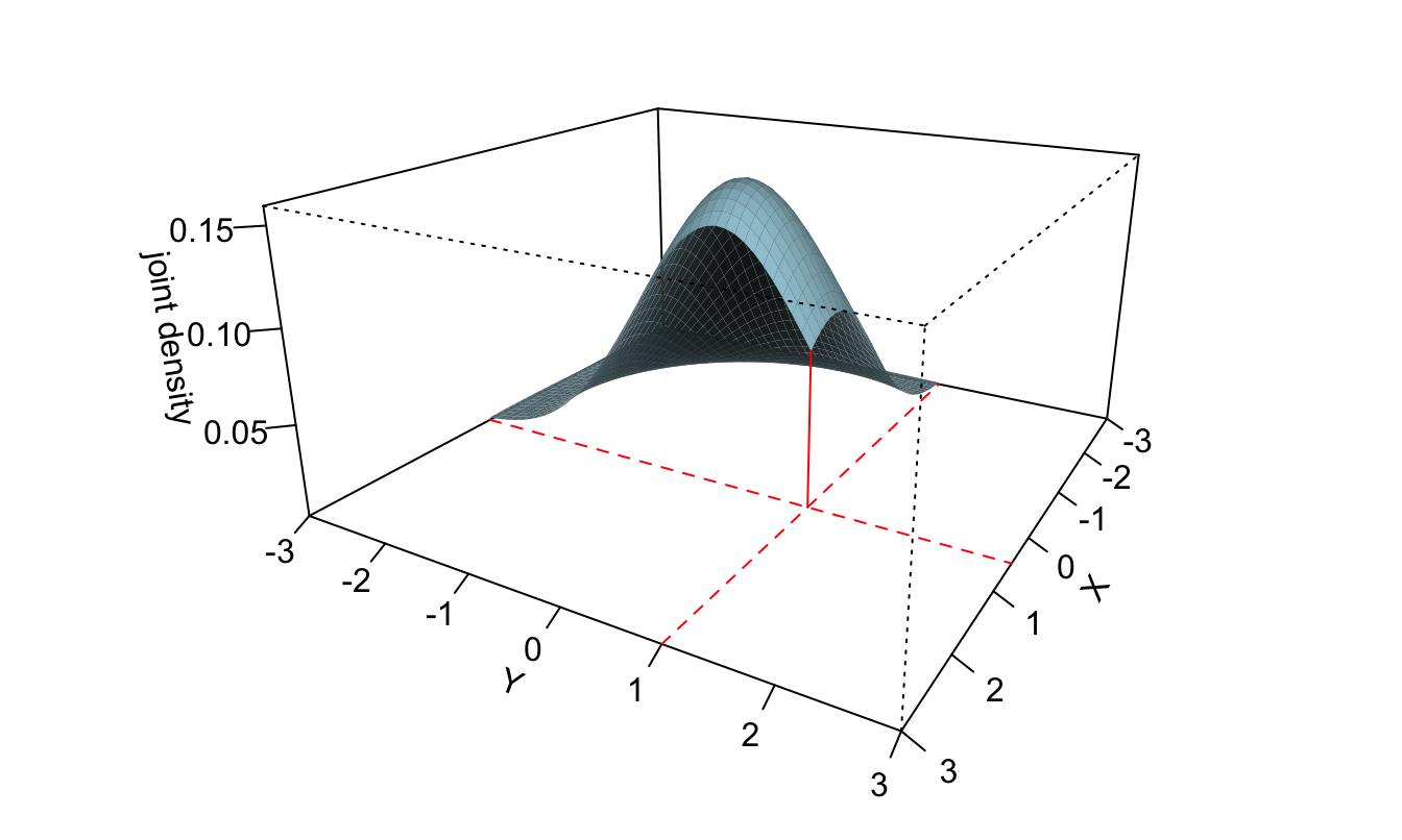
Figure 1.1: The volume between the horizontal plane (\(z=0\)) and the surface is equal to \(F_{XY}(0.5,1)=\mathbb{P}(X<0.5,Y<1)\).

Definition 1.4 (Joint probability density function (p.d.f.)) The continuous random variables \(X\) and \(Y\) admit the joint p.d.f. \(f_{XY}\), where \(f_{XY}(x,y) \ge 0\) for all \(x\) and \(y\), if: \[ \mathbb{P}(a < X \le b,c < Y \le d) = \int_{a}^{b}\int_{c}^{d}f_{XY}(x,y)dy dx, \quad \forall a \le b,\;c \le d. \]

The marginal density is the continuous counterpart of a column or row total: \[ f_X(x)=\int_{-\infty}^{+\infty}f_{XY}(x,y)dy, \qquad f_Y(y)=\int_{-\infty}^{+\infty}f_{XY}(x,y)dx. \]

In particular, we have: \[\begin{eqnarray*} &&f_{XY}(x,y)\\ &=& \lim_{\varepsilon \rightarrow 0} \frac{\mathbb{P}(x < X \le x + \varepsilon,y < Y \le y + \varepsilon)}{\varepsilon^2} \\ &=& \lim_{\varepsilon \rightarrow 0} \frac{F_{XY}(x + \varepsilon,y + \varepsilon)-F_{XY}(x,y + \varepsilon)-F_{XY}(x + \varepsilon,y)+F_{XY}(x,y)}{\varepsilon^2}. \end{eqnarray*}\]

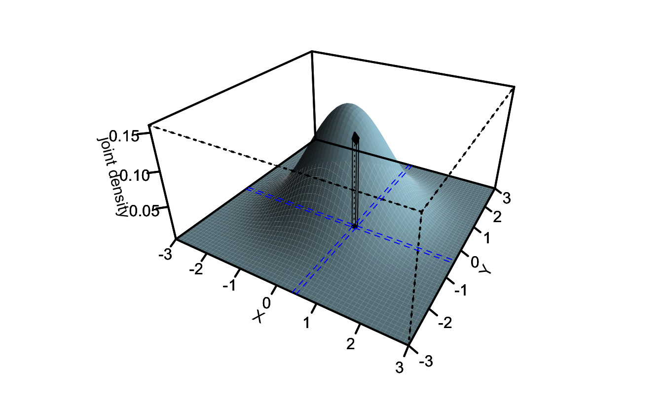
Figure 1.2: Assume that the basis of the black column is defined by those points whose \(x\)-coordinates are between \(x\) and \(x+\varepsilon\) and \(y\)-coordinates are between \(y\) and \(y+\varepsilon\). Then the volume of the black column is equal to \(\mathbb{P}(x < X \le x+\varepsilon,y < Y \le y+\varepsilon)\), which is approximately equal to \(f_{XY}(x,y)\varepsilon^2\) if \(\varepsilon\) is small.

Figure 1.3 illustrates why we have \[\begin{eqnarray*} &&\mathbb{P}(x < X \le x + \varepsilon,y < Y \le y + \varepsilon)\\ &=& F_{XY}(x + \varepsilon,y + \varepsilon)-F_{XY}(x,y + \varepsilon)-F_{XY}(x + \varepsilon,y)+F_{XY}(x,y). \end{eqnarray*}\] Let us denote by \(P_\Omega\) the probability that the point of coordinate \((X,Y)\) is included in the \(\Omega\) area. We have: \[ P_{B} = P_{B+C+D+E} - P_{E+D} - P_{E+C} + P_E, \] which implies that \[\begin{eqnarray*} &&\mathbb{P}(x<X\le x+ \varepsilon,y<Y\le y+ \varepsilon) \\ &=& \mathbb{P}(X\le x+ \varepsilon,Y\le y+ \varepsilon) - \mathbb{P}(X\le x+ \varepsilon,Y\le y) - \mathbb{P}(X\le x,Y\le y+ \varepsilon)\\ &&+ \mathbb{P}(X\le x,Y\le y). \end{eqnarray*}\]

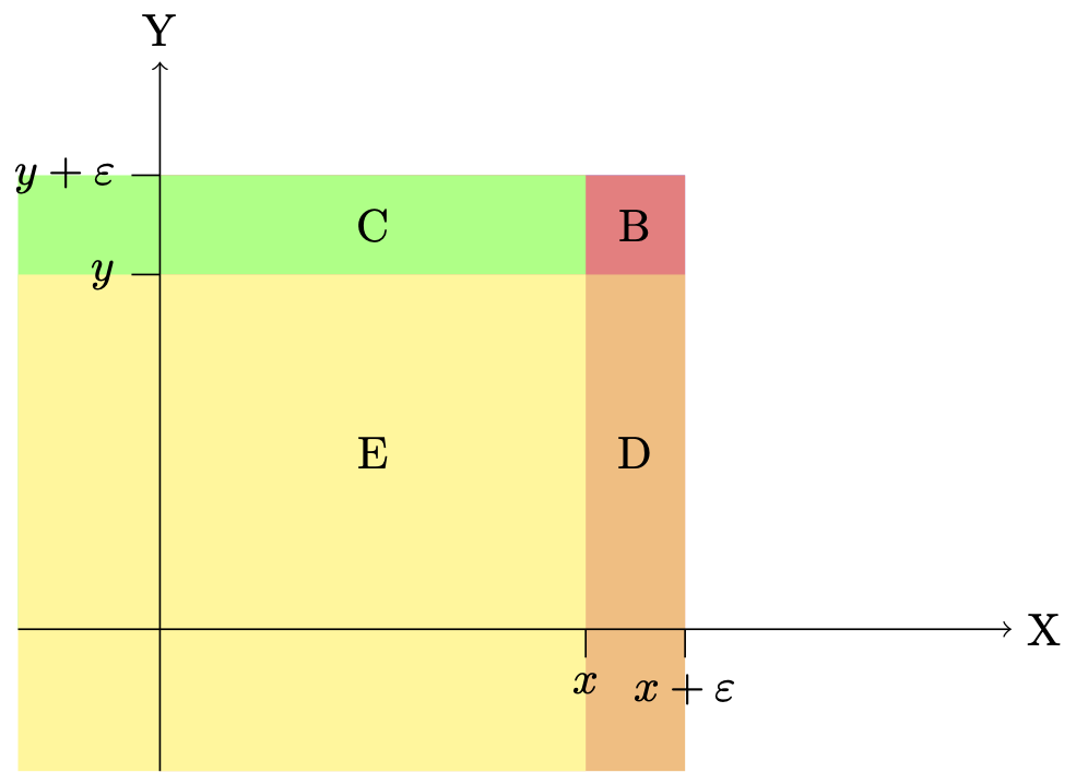
Figure 1.3: Area \(B+C+D+E\) encompasses the points with coordinates \((X,Y)\) such that \(X\le x+\varepsilon\) and \(Y \le y + \varepsilon\). Area \(D+E\) encompasses the points with coordinates \((X,Y)\) such that \(X\le x+\varepsilon\) and \(Y \le y\). Area \(C+E\) encompasses the points with coordinates \((X,Y)\) such that \(X\le x\) and \(Y \le y + \varepsilon\).

Definition 1.5 (Conditional probability density function) If \(X\) and \(Y\) are continuous random variables and \(f_Y(y)>0\), the conditional density of \(X\) given \(Y=y\) is denoted by \(f_{X|Y}(x,y)\).

It describes the distribution of \(X\) within the subpopulation characterized by \(Y=y\). The associated conditional expectation is \[ \mathbb{E}(X\mid Y=y)=\int_{-\infty}^{+\infty}x f_{X|Y}(x,y)dx. \]

Proposition 1.1 (Conditional density) We have \[ f_{X|Y}(x,y)=\frac{f_{XY}(x,y)}{f_Y(y)}. \]

Proof. Condition on a shrinking interval around \(y\). Then \[\begin{eqnarray*} f_{X|Y}(x,y) &=&\lim_{\varepsilon,\delta \rightarrow 0} \frac{\mathbb{P}(x<X\le x+\varepsilon\mid y<Y\le y+\delta)}{\varepsilon}\\ &=&\lim_{\varepsilon,\delta \rightarrow 0} \frac{\mathbb{P}(x<X\le x+\varepsilon,y<Y\le y+\delta)} {\varepsilon\,\mathbb{P}(y<Y\le y+\delta)}\\ &=&\frac{f_{XY}(x,y)}{f_Y(y)}. \end{eqnarray*}\]

Definition 1.6 (Independent random variables) Consider two r.v., \(X\) and \(Y\), with respective c.d.f. \(F_X\) and \(F_Y\), and respective p.d.f. \(f_X\) and \(f_Y\).

These random variables are independent if and only if (iff) the joint c.d.f. of \(X\) and \(Y\) (see Def. 1.3) is given by: \[ F_{XY}(x,y) = F_{X}(x) \times F_{Y}(y), \] or, equivalently, iff the joint p.d.f. of \((X,Y)\) (see Def. 1.4) is given by: \[ f_{XY}(x,y) = f_{X}(x) \times f_{Y}(y). \]

We have the following:

1. If \(X\) and \(Y\) are independent, \(f_{X|Y}(x,y)=f_{X}(x)\). This implies, in particular, that \(\mathbb{E}(g(X)|Y)=\mathbb{E}(g(X))\), where \(g\) is any function.
2. If \(X\) and \(Y\) are independent, then \(\mathbb{E}(g(X)h(Y))=\mathbb{E}(g(X))\mathbb{E}(h(Y))\) and \(\mathbb{C}ov(g(X),h(Y))=0\), where \(g\) and \(h\) are any functions.

It is important to note that the absence of correlation between two variables is not a sufficient condition to have independence. Consider for instance the case where \(X=Y^2\), with \(Y \sim\mathcal{N}(0,1)\). In this case, we have \(\mathbb{C}ov(X,Y)=0\), but \(X\) and \(Y\) are not independent. Indeed, we have for instance \(\mathbb{E}(Y^2 \times X)=3\), which is not equal to \(\mathbb{E}(Y^2) \times \mathbb{E}(X)=1\). (If \(X\) and \(Y\) were independent, we should have \(\mathbb{E}(Y^2 \times X)=\mathbb{E}(Y^2) \times \mathbb{E}(X)\) according to point 2 above.)

The correspondence between the two settings can be summarized as follows:

Concept	Discrete variables	Continuous variables
Distribution	probabilities \(p_X(x)\)	density \(f_X(x)\)
Marginalization	sum joint probabilities	integrate the joint density
Conditioning	divide by a marginal probability	divide by a marginal density
Expectation	probability-weighted sum	density-weighted integral

Practice: Exercise 1.4 asks how a density changes after conditioning above a quantile.

1.4 Law of iterated expectations

The conditional means describe different subpopulations. To recover the population mean, we average those conditional means using the population shares of the groups.

Proposition 1.2 (Law of iterated expectations) If \(X\) and \(Y\) are two random variables and if \(\mathbb{E}(|X|)<\infty\), we have: \[ \boxed{\mathbb{E}(X) = \mathbb{E}(\mathbb{E}(X|Y)).} \]

Proof. Suppose first that both \(X\) and \(Y\) are discrete. Partitioning the population according to the possible values of \(Y\) gives \[\begin{eqnarray*} \mathbb{E}(X) &=&\sum_x x\mathbb{P}(X=x)\\ &=&\sum_x x\sum_y\mathbb{P}(X=x\mid Y=y)\mathbb{P}(Y=y)\\ &=&\sum_y\left[\sum_x x\mathbb{P}(X=x\mid Y=y)\right]\mathbb{P}(Y=y)\\ &=&\sum_y\mathbb{E}(X\mid Y=y)\mathbb{P}(Y=y) =\mathbb{E}[\mathbb{E}(X\mid Y)]. \end{eqnarray*}\] For continuous \(Y\), the same argument applies with integrals replacing sums.

In Example 1.2, the population mean commuting time is therefore \[ \mathbb{E}(X) =1.2\times 0.5+0.5\times 0.5 =0.85. \] We obtain the same value directly from the marginal distribution of \(X\): \[ \mathbb{E}(X)=0\times0.40+1\times0.35+2\times0.25=0.85. \]

The first calculation averages across groups; the second averages across commuting-time outcomes. The law of iterated expectations states that these two routes must agree.

Example 1.3 (Mixture of Gaussian distributions) By definition, \(X\) is drawn from a mixture of Gaussian distributions if: \[ X = \color{blue}{B \times Y_1} + \color{red}{(1-B) \times Y_2}, \] where \(B\), \(Y_1\) and \(Y_2\) are three independent variables drawn as follows: \[ B \sim \mbox{Bernoulli}(p),\quad Y_1 \sim \mathcal{N}(\mu_1,\sigma_1^2), \quad \mbox{and}\quad Y_2 \sim \mathcal{N}(\mu_2,\sigma_2^2). \]

Figure 1.4 displays the densities of three Gaussian mixtures. This web interface can be used to explore other parameter values.

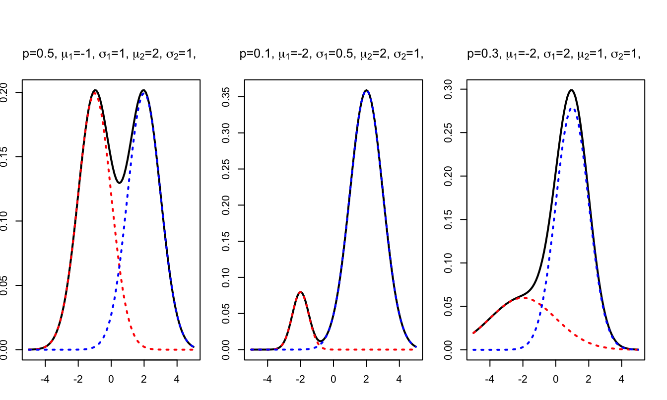
Figure 1.4: Example of pdfs of mixtures of Gaussian distribututions.

The law of iterated expectations gives: \[ \mathbb{E}(X) = \mathbb{E}(\mathbb{E}(X|B)) = \mathbb{E}(B\mu_1+(1-B)\mu_2)=p\mu_1 + (1-p)\mu_2. \]

Example 1.4 (Buffon (1733)'s needles) Suppose we have a floor made of parallel strips of wood, each the same width [\(w=1\)]. We drop a needle, of length \(1/2\), onto the floor. What is the probability that the needle crosses the grooves of the floor?

Let’s define the random variable \(X\) by \[ X = \left\{ \begin{array}{cl} 1 & \mbox{if the needle crosses a line}\\ 0 & \mbox{otherwise.} \end{array} \right. \] Conditionally on \(\theta\), it can be seen that we have \(\mathbb{E}(X|\theta)=\cos(\theta)/2\) (see Figure 1.5).

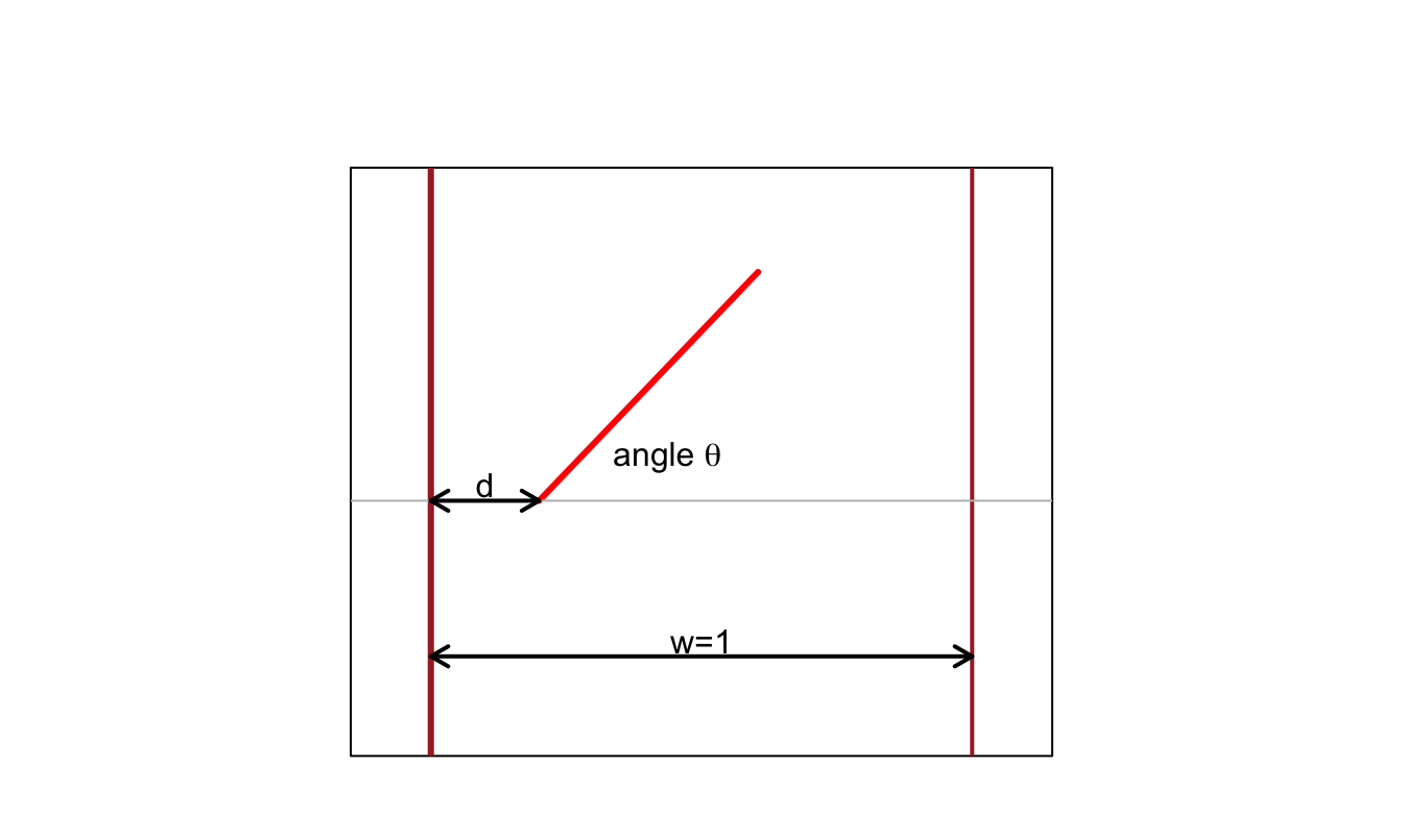
Figure 1.5: Schematic representation of the problem.

It is reasonable to assume that \(\theta\) is uniformly distributed on \([-\pi/2,\pi/2]\), therefore: \[ \mathbb{E}(X)=\mathbb{E}(\mathbb{E}(X|\theta))=\mathbb{E}(\cos(\theta)/2)=\int_{-\pi/2}^{\pi/2}\frac{1}{2}\cos(\theta)\left(\frac{d\theta}{\pi}\right)=\frac{1}{\pi}. \]

This web interface simulates the experiment (select the worksheet “Buffon’s needles”).

Practice: Exercise 1.7 distinguishes conditional and unconditional moments.

1.5 Law of total variance

The population variance also has a useful group interpretation. It combines average dispersion within groups and dispersion between group means.

Proposition 1.3 (Law of total variance) If \(X\) and \(Y\) are two random variables and if the variance of \(X\) is finite, we have: \[ \boxed{\mathbb{V}ar(X) = \mathbb{E}(\mathbb{V}ar(X|Y)) + \mathbb{V}ar(\mathbb{E}(X|Y)).} \]

Proof. We have: \[\begin{eqnarray*} \mathbb{V}ar(X) &=& \mathbb{E}(X^2) - \mathbb{E}(X)^2\\ &=& \mathbb{E}(\mathbb{E}(X^2|Y)) - \mathbb{E}(X)^2\\ &=& \mathbb{E}(\mathbb{E}(X^2|Y) \color{blue}{- \mathbb{E}(X|Y)^2}) + \color{blue}{\mathbb{E}(\mathbb{E}(X|Y)^2)} - \color{red}{\mathbb{E}(X)^2}\\ &=& \mathbb{E}(\underbrace{\mathbb{E}(X^2|Y) - \mathbb{E}(X|Y)^2}_{\mathbb{V}ar(X|Y)}) + \underbrace{\mathbb{E}(\mathbb{E}(X|Y)^2) - \color{red}{\mathbb{E}(\mathbb{E}(X|Y))^2}}_{\mathbb{V}ar(\mathbb{E}(X|Y))}. \end{eqnarray*}\]

Returning to Example 1.2, one obtains \[ \mathbb{V}ar(X\mid Y=0)=0.56,\qquad \mathbb{V}ar(X\mid Y=1)=0.45. \] Consequently, \[ \underbrace{\mathbb{E}[\mathbb{V}ar(X\mid Y)]}_{\text{within-group variation}} =0.505, \qquad \underbrace{\mathbb{V}ar[\mathbb{E}(X\mid Y)]}_{\text{between-group variation}} =0.1225. \] The total variance is \(0.505+0.1225=0.6275\). This decomposition is often useful in economics because it separates heterogeneity within observable groups from differences in their average outcomes.

Example 1.5 (Mixture of Gaussian distributions (cont'd)) Consider the case of a mixture of Gaussian distributions (Example 1.3). We have: \[\begin{eqnarray*} \mathbb{V}ar(X) &=& \color{blue}{\mathbb{E}(\mathbb{V}ar(X|B))} + \color{red}{\mathbb{V}ar(\mathbb{E}(X|B))}\\ &=& \color{blue}{p\sigma_1^2+(1-p)\sigma_2^2} + \color{red}{p(1-p)(\mu_1 - \mu_2)^2}. \end{eqnarray*}\]

Practice: Exercise 1.3 separates within-group and between-group variation.

1.6 Bias, accuracy, and consistency

The quantities introduced so far—means, variances, and probabilities—describe a population. In applications, these quantities are usually unknown and must be estimated from a sample.

Let \(X_1,\ldots,X_n\) be an independent and identically distributed sample from a population with mean \(\mu\) and finite variance \(\sigma^2\). The sample mean \[ \overline X_n=\frac{1}{n}\sum_{i=1}^n X_i \] is an estimator of \(\mu\). It satisfies \[ \mathbb{E}(\overline X_n)=\mu, \qquad \mathbb{V}ar(\overline X_n)=\frac{\sigma^2}{n}. \] Thus its distribution is centred on the population mean and becomes increasingly concentrated as the sample grows. This example anticipates three properties used to evaluate estimators: bias, precision, and consistency.

More generally, let \(\widehat\theta\) estimate a fixed parameter \(\theta\). Its bias is \(\mathbb{E}(\widehat\theta)-\theta\); an unbiased estimator has zero bias. When its second moment is finite, its mean squared error satisfies \[ \operatorname{MSE}(\widehat\theta)=\mathbb{E}[(\widehat\theta-\theta)^2] =\mathbb{V}ar(\widehat\theta)+\operatorname{Bias}(\widehat\theta)^2. \] A small variance means the estimator is concentrated around its own mean; it does not guarantee that this mean is close to the parameter. Exercise 1.5 derives this decomposition. Consistency concerns a different question: what happens as the sample grows?

Econometric parameters include causal effects, elasticities, distributional parameters, and preference parameters such as risk aversion. Except in degenerate cases, an estimate differs from its population target in any particular sample. Consistency requires the estimator to approach that target as the sample size increases.

Denote by \(\hat\theta_n\) the estimate of \(\theta\) based on a sample of size \(n\). We say that \(\hat\theta\) is a consistent estimator of \(\theta\) if, for any \(\varepsilon>0\) (even if very small), the probability that \(\hat\theta_n\) is in \([\theta - \varepsilon,\theta + \varepsilon]\) goes to 1 when \(n\) goes to \(\infty\). Formally: \[ \lim_{n \rightarrow + \infty} \mathbb{P}\left(\hat\theta_n \in [\theta - \varepsilon,\theta + \varepsilon]\right) = 1. \]

That is, \(\hat\theta\) is a consistent estimator if \(\hat\theta_n\) converges in probability (Def. 9.16) to \(\theta\). The sample mean above is consistent when the observations have a finite variance, because \(\mathbb{V}ar(\overline X_n)=\sigma^2/n\) converges to zero. There are also other types of stochastic convergence.¹

Example 1.6 (Example of non-convergent estimator) Assume that \(X_i \sim i.i.d. \mbox{Cauchy}\) with a location parameter of 1 and a scale parameter of 1 (Def. 9.14). The sample mean \(\bar{X}_n = \frac{1}{n}\sum_{i=1}^{n} X_i\) does not converge in probability. This is because a Cauchy distribution has no mean; hence the law of large numbers (Theorem 2.1) does not apply.

The realization below is especially deceptive. For several thousand observations, the sample mean appears to settle near the location parameter 1. But observation 4,495 is approximately 75,073: it moves the sample mean from about 1.01 to 17.71. Increasing the sample size has not protected the sample mean against a new extreme Cauchy draw.

Code

set.seed(7221) # Reproducible path with a late extreme observation
N <- 5000
X <- rcauchy(N, location=1)
X.bar <- cumsum(X)/(1:N)
par(mfrow=c(1,2), mar=c(4.2,5.2,2.6,1),
    mgp=c(2.5,.8,0), las=1, cex.axis=.85)
plot(X,type="l",xlab="sample size (n)",
     ylab="",main=expression(X[n]),lwd=2)
plot(X.bar,type="l",xlab="sample size (n)",
     ylab="",main=expression(bar(X)[n]),lwd=2)
abline(h=1,lty=2,col="grey")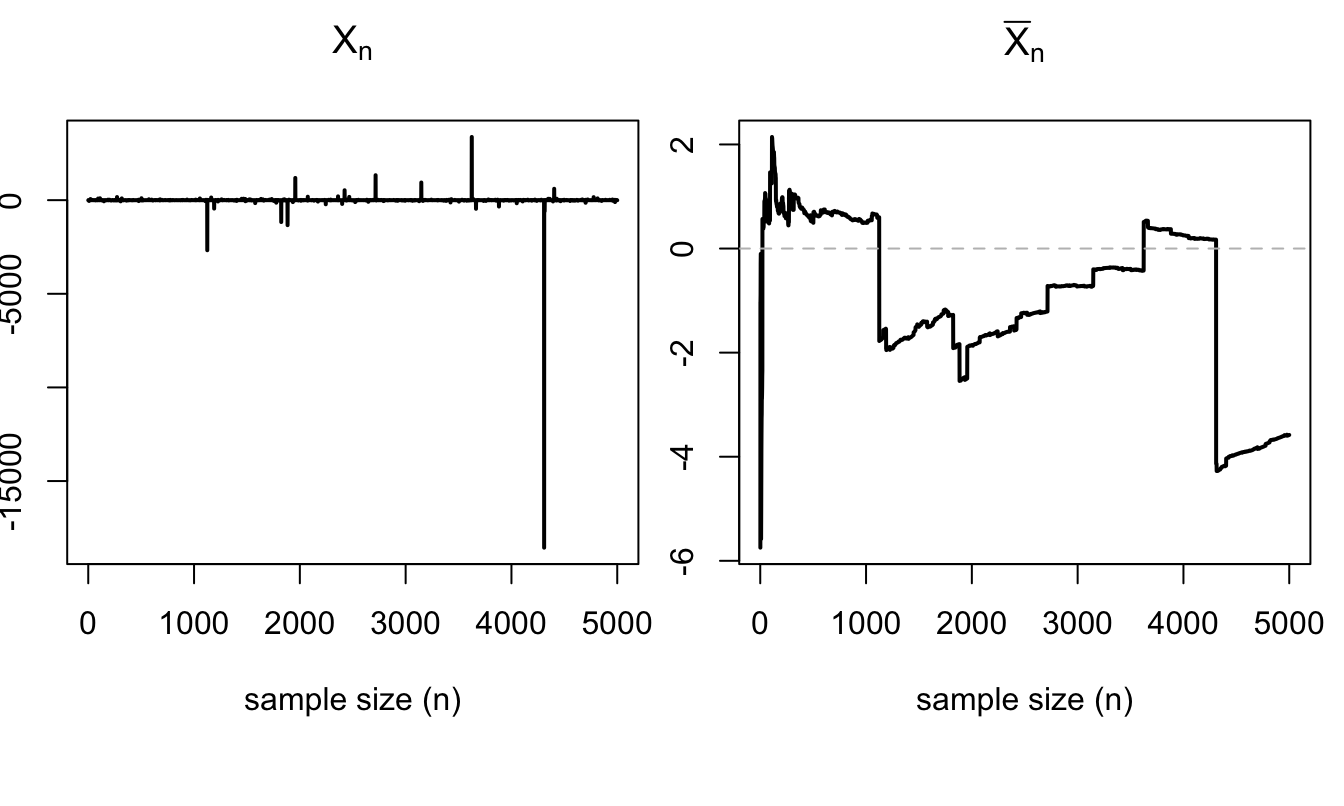

Figure 1.6: Simulation of \(\bar{X}_n\) when \(X_i \sim i.i.d. \mbox{Cauchy}\).

1.7 Chapter recap

• Moments summarize the location, dispersion, and co-movement of random variables; Section 1.1 introduces expectation, variance, and covariance.
• A joint distribution determines marginal and conditional distributions. Example 1.2 illustrates these operations for discrete variables, while Proposition 1.1 gives the continuous conditional-density formula.
• Bayes’ rule in Section 1.2.2 reverses the direction of conditioning; Definition 1.6 states when conditioning leaves a distribution unchanged.
• Proposition 1.2 recovers a population mean by averaging conditional means.
• Proposition 1.3 decomposes population variance into within-group and between-group components.
• Section 1.6 distinguishes finite-sample bias and precision from consistency as the sample size grows.

1.8 Exercises

Attempt each question and explain your reasoning, including for true-or-false statements. Foundation exercises apply a result directly; Standard exercises require several steps or a short proof; Advanced exercises combine several results or require a longer derivation. Worked solutions and exercise-specific hints are reserved for teaching sessions and are not included in this student edition.

Exercise 1.1 (Covariance identities) Standard | Analytical
Review Section 1.1.

Let \(X,Y,V\) have finite second moments, and let \(a,b,c\) be constants. Write \(\mu_X=\mathbb{E}(X)\) and \(\sigma_{XY}=\mathbb{C}ov(X,Y)\).

1. Show that \(\mathbb{C}ov(a+bX+cV,Y)=b\sigma_{XY}+c\sigma_{VY}\).
2. Show that \(\mathbb{E}(XY)=\mathbb{C}ov(X,Y)+\mathbb{E}(X)\mathbb{E}(Y)\).

Exercise 1.2 (Bayes rule and facial recognition) Foundation | Calculation
Review Section 1.2.2.

A security system grants access to an authorized person with probability \(0.99\), and to an unauthorized person with probability \(0.02\). Of those attempting to enter, \(5\%\) are unauthorized.

1. Given that a person is granted access, what is the probability that the person is authorized?
2. Given that a person is denied access, what is the probability that the person is unauthorized?

Exercise 1.3 (Within-group and between-group variation) Foundation | Calculation
Review Section 1.5.

Let \(X\) be daily time spent on social media (in hours), and let \(Y\) indicate age group. The population has the following characteristics:

Age group	Share	Mean (h)	Variance (\(\mathrm{h}^2\))
Under 30	0.6	4	1.5
30 or above	0.4	2	0.5

1. Calculate \(\mathbb{E}[\mathbb{V}ar(X\mid Y)]\).
2. Calculate \(\mathbb{E}[\mathbb{E}(X\mid Y)]\).
3. Calculate \(\mathbb{V}ar[\mathbb{E}(X\mid Y)]\).
4. Use the law of total variance to obtain \(\mathbb{V}ar(X)\).

Exercise 1.4 (Conditioning above a quantile) Standard | Analytical
Review Section 1.3.

Let \(X\) have a continuous density \(f\) and cumulative distribution function \(F\). For \(0<\alpha<1\), let \(q_\alpha\) satisfy \(F(q_\alpha)=\alpha\).

1. How can \(f\) be obtained from \(F\)?
2. Derive the c.d.f. \(F_\alpha\) of \(X\) conditional on \(X>q_\alpha\). State its value both below and above \(q_\alpha\).
3. Derive the corresponding density \(f_\alpha\).

Exercise 1.5 (Bias, variance, and mean squared error) Standard | Analytical
Review Section 1.6.

Let \(\widehat\theta\) estimate a fixed parameter \(\theta\), and suppose \(\widehat\theta\) has a finite second moment.

1. What property is expressed by \(\mathbb{E}(\widehat\theta)=\theta\)?
2. Express \(\mathbb{E}[(\widehat\theta-\theta)^2]\) in terms of the variance and bias of \(\widehat\theta\).
3. Does a small variance necessarily imply a small mean squared error? Explain.

Exercise 1.6 (Employment, residence, and independence) Standard | Calculation
Review Section 1.2.

Let \(X\) indicate employment status (\(0\): employed; \(1\): self-employed), and let \(Y\) indicate residence (\(0\): countryside; \(1\): city). Their joint probabilities are:

	\(Y=0\)	\(Y=1\)
\(X=0\)	0.10	0.30
\(X=1\)	0.15	0.45

For each statement, decide whether it is true or false and justify your answer.

1. \(\mathbb{E}(X)=0.7\).
2. \(X\) and \(Y\) are not independent.
3. \(\mathbb{V}ar(X)=\mathbb{V}ar(X\mid Y=0)+\mathbb{V}ar(X\mid Y=1)\).
4. \(\mathbb{V}ar(X\mid Y=0)=0.24\).
5. Bayes’ rule implies \[ \begin{gathered} \mathbb{P}(X=0\mid Y=0)\\ =\frac{\mathbb{P}(Y=0\mid X=0)\mathbb{P}(X=0)} {\mathbb{P}(Y=0\mid X=0)\mathbb{P}(X=0)+\mathbb{P}(Y=0\mid X=1)\mathbb{P}(X=1)}. \end{gathered} \]
6. The correlation between \(X\) and \(Y\) is strictly positive.

Exercise 1.7 (A Bernoulli variable with a random success probability) Standard | Analytical
Review Section 1.4.

Let \(U\) be uniform on \([0,1]\), and suppose \(Y\mid U\sim\operatorname{Bernoulli}(U)\).

For each statement, decide whether it is true or false and justify your answer.

1. \(\mathbb{E}(Y\mid U)=U\).
2. \(\mathbb{V}ar(Y\mid U)=U^2\).
3. \(\mathbb{V}ar(Y)=1/4\).
4. \(\mathbb{E}(Y)=1/4\).
5. \(\mathbb{E}(Y+U)=2U\).

---

1. Appendix 9.3.3 notably provides the definitions of convergence in distribution (Def. 9.19) and mean-square convergence (Def. 9.17).↩︎