5 Panel regressions
5.1 Specification and notations
A standard panel situation is as follows: the sample covers a lot of “entities”, indexed by \(i \in \{1,\dots,n\}\), with \(n\) large, and, for each entity, we observe different variables over a small number of periods \(t \in \{1,\dots,T\}\). This is a longitudinal dataset.
The linear panel regression model is: \[\begin{equation} y_{i,t} = \mathbf{x}'_{i,t}\underbrace{\boldsymbol\beta}_{K \times 1} + \underbrace{\mathbf{z}'_{i}\boldsymbol\alpha}_{\mbox{Individual effects}} + \varepsilon_{i,t}.\tag{5.1} \end{equation}\]
When running panel regressions, the usual objective is to estimate \(\boldsymbol\beta\).
Figure 5.1 illustrates a panel-data situation. The model is \(y_i = \alpha_i + \beta x_{i,t} + \varepsilon_{i,t}\), \(t \in \{1,2\}\). On Panel (b), blue dots are for \(t=1\), red dots are for \(t=2\). The lines relate the dots associated with the same entity \(i\). What is remarkable in the simulated model is that, while the unconditional correlation between \(y\) and \(x\) is negative, the conditional correlation (conditional on \(\alpha_i\)) is positive. Indeed, the sign of this conditional correlation is the sign of \(\beta\), which is positive in th simulated example (\(\beta=5\)). In other words, if one did not know the panel nature of the data, that would be tempting to say that \(\beta<0\), but this is not the case, due to fixed effects (the \(\alpha_i\)’s) that are negatively correlated to the \(x_i\)’s.
T <- 2; n <- 12 # 2 periods and 12 entities
alpha <- 5*rnorm(n) # draw fixed effects
x.1 <- rnorm(n) - .5*alpha # note: x_i's correlate to alpha_i's
x.2 <- rnorm(n) - .5*alpha
beta <- 5; sigma <- .3
y.1 <- alpha + x.1 + sigma*rnorm(n);y.2 <- alpha + x.2 + sigma*rnorm(n)
x <- c(x.1,x.2) # pooled x
y <- c(y.1,y.2) # pooled y
par(mfrow=c(1,2))
plot(x,y,col="black",pch=19,xlab="x",ylab="y",main="(a)")
plot(x,y,col="black",pch=19,xlab="x",ylab="y",main="(b)")
points(x.1,y.1,col="blue",pch=19);points(x.2,y.2,col="red",pch=19)
for(i in 1:n){lines(c(x.1[i],x.2[i]),c(y.1[i],y.2[i]))}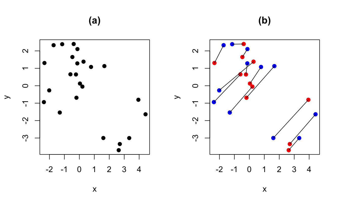
Figure 5.1: The data are the same for both panels. On Panel (b), blue dots are for \(t=1\), red dots are for \(t=2\). The lines relate the dots associated to the same entity \(i\).
Figure 5.2 presents the same type of plot based on the Cigarette Consumption Panel dataset (CigarettesSW dataset, used in J. Stock and Watson (2003)). This dataset documents the average consumption of cigarettes in 48 continental US states for two dates (1985 and 1995).
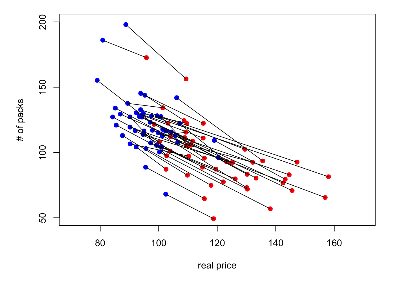
Figure 5.2: Cigarette consumption versus real price in the CigarettesSW panel dataset.
We will make use of the following notations: \[ \mathbf{y}_i = \underbrace{\left[ \begin{array}{c} y_{i,1}\\ \vdots\\ y_{i,T} \end{array}\right]}_{T \times 1}, \quad \boldsymbol\varepsilon_i = \underbrace{\left[ \begin{array}{c} \varepsilon_{i,1}\\ \vdots\\ \varepsilon_{i,T} \end{array}\right]}_{T \times 1}, \quad \mathbf{x}_i = \underbrace{\left[ \begin{array}{c} \mathbf{x}_{i,1}'\\ \vdots\\ \mathbf{x}_{i,T}' \end{array}\right]}_{T \times K}, \quad \mathbf{X} = \underbrace{\left[ \begin{array}{c} \mathbf{x}_{1}\\ \vdots\\ \mathbf{x}_{n} \end{array}\right]}_{(nT) \times K}. \] \[ \tilde{\mathbf{y}}_i = \left[ \begin{array}{c} y_{i,1} - \bar{y}_i\\ \vdots\\ y_{i,T} - \bar{y}_i \end{array}\right], \quad \tilde{\boldsymbol\varepsilon}_i = \left[ \begin{array}{c} \varepsilon_{i,1} - \bar{\varepsilon}_i\\ \vdots\\ \varepsilon_{i,T} - \bar{\varepsilon}_i \end{array}\right], \] \[ \tilde{\mathbf{x}}_i = \left[ \begin{array}{c} \mathbf{x}_{i,1}' - \bar{\mathbf{x}}_i'\\ \vdots\\ \mathbf{x}_{i,T}' - \bar{\mathbf{x}}_i' \end{array}\right], \quad \tilde{\mathbf{X}} = \left[ \begin{array}{c} \tilde{\mathbf{x}}_{1}\\ \vdots\\ \tilde{\mathbf{x}}_{n} \end{array}\right], \quad \tilde{\mathbf{Y}} = \left[ \begin{array}{c} \tilde{\mathbf{y}}_{1}\\ \vdots\\ \tilde{\mathbf{y}}_{n} \end{array}\right], \] where \[ \bar{y}_i = \frac{1}{T} \sum_{t=1}^T y_{i,t}, \quad \bar{\varepsilon}_i = \frac{1}{T}\sum_{t=1}^T \varepsilon_{i,t} \quad \mbox{and} \quad \bar{\mathbf{x}}_i = \frac{1}{T}\sum_{t=1}^T \mathbf{x}_{i,t}. \]
5.2 Three standard cases
There are three typical situations:
- Pooled regression: \(\mathbf{z}_i \equiv 1\). This case amounts to the case studied in Chapter 4.
- Fixed Effects (Section 5.3): \(\mathbf{z}_i\) is unobserved, but correlates with \(\mathbf{x}_i\) \(\Rightarrow\) \(\mathbf{b}\) is biased and inconsistent in the OLS regression of \(\mathbf{y}\) on \(\mathbf{X}\) (omitted variable, see Section 4.3.2).
- Random Effects (Section 5.4): \(\mathbf{z}_i\) is unobserved, but uncorrelated with \(\mathbf{x}_i\). The model writes: \[ y_{i,t} = \mathbf{x}'_{i,t}\boldsymbol\beta + \alpha + \underbrace{{\color{blue}u_i + \varepsilon_{i,t}}}_{\mbox{compound error}}, \] where \(\alpha = \mathbb{E}(\mathbf{z}'_{i}\boldsymbol\alpha)\) and \(u_i = \mathbf{z}'_{i}\boldsymbol\alpha - \mathbb{E}(\mathbf{z}'_{i}\boldsymbol\alpha) \perp \mathbf{x}_i\). In that case, the OLS is consistent, but not efficient. GLS can be used to gain efficiencies over OLS (see Section 4.5.2 for a presentation of the GLS approach).
5.3 Estimation of Fixed-Effects Models
Hypothesis 5.1 (Fixed-effect model) We assume that:
- There is no perfect multicollinearity among the regressors.
- \(\mathbb{E}(\varepsilon_{i,t}|\mathbf{X})=0\), for all \(i,t\).
- We have: \[ \mathbb{E}(\varepsilon_{i,t}\varepsilon_{j,s}|\mathbf{X}) = \left\{ \begin{array}{cl} \sigma^2 & \mbox{if $i=j$ and $s=t$},\\ 0 & \mbox{otherwise.} \end{array}\right. \]
These assumptions are analogous to those introduced in the standard linear regression:
- \(\leftrightarrow\) Hyp. 4.1, (ii) \(\leftrightarrow\) Hyp. 4.2, (iii) \(\leftrightarrow\) Hyp. 4.3 + 4.4.
In matrix form, for a given \(i\), the model writes: \[ \mathbf{y}_i = \mathbf{x}_i \boldsymbol\beta + \mathbf{1}_T\alpha_i + \boldsymbol\varepsilon_i, \] where \(\mathbf{1}_T\) is a \(T\)-dimensional vector of ones.
This is the Least Square Dummy Variable (LSDV) model: \[\begin{equation} \mathbf{y} = [\mathbf{X} \quad \mathbf{D}] \left[ \begin{array}{c} \boldsymbol\beta\\ \boldsymbol\alpha \end{array} \right] + \boldsymbol\varepsilon, \tag{5.2} \end{equation}\] with: \[ \mathbf{D} = \underbrace{ \left[\begin{array}{cccc} \mathbf{1}_T&\mathbf{0}&\dots&\mathbf{0}\\ \mathbf{0}&\mathbf{1}_T&\dots&\mathbf{0}\\ &&\vdots&\\ \mathbf{0}&\mathbf{0}&\dots&\mathbf{1}_T\\ \end{array}\right]}_{(nT \times n)}. \]
The linear regression (Eq. (5.2)) —with the dummy variables— satisfies the Gauss-Markov conditions (Theorem 4.1). Hence, in this context, the OLS estimator is the best linear unbiased estimator (BLUE).
Denoting by \(\mathbf{Z}\) the matrix \([\mathbf{X} \quad \mathbf{D}]\), and by \(\mathbf{b}\) and \(\mathbf{a}\) the respective OLS estimates of \(\boldsymbol\beta\) and of \(\boldsymbol\alpha\), we have: \[\begin{equation} \boxed{ \left[ \begin{array}{c} \mathbf{b}\\ \mathbf{a} \end{array} \right] = [\mathbf{Z}'\mathbf{Z}]^{-1}\mathbf{Z}'\mathbf{y}.} \tag{5.3} \end{equation}\]
The asymptotical distribution of \([\mathbf{b}',\mathbf{a}']'\) derives from the standard OLS context: Prop. 4.11 can be used after having replaced \(\mathbf{X}\) by \(\mathbf{Z}=[\mathbf{X} \quad \mathbf{D}]\).
We have: \[\begin{equation} \boxed{\left[ \begin{array}{c} \mathbf{b}\\ \mathbf{a} \end{array} \right] \overset{d}{\rightarrow} \mathcal{N}\left( \left[ \begin{array}{c} \boldsymbol\beta\\ \boldsymbol\alpha \end{array} \right], \sigma^2 \frac{Q^{-1}}{nT} \right),} \end{equation}\] where \[ Q = \mbox{plim}_{nT \rightarrow \infty} \frac{1}{nT} \mathbf{Z}'\mathbf{Z}, \] assuming the previous limit exists.
In practice, an estimator of the covariance matrix of \([\mathbf{b}',\mathbf{a}']'\) is: \[ s^2 \left( \mathbf{Z}'\mathbf{Z}\right)^{-1} \quad with \quad s^2 = \frac{\mathbf{e}'\mathbf{e}}{nT - K - n}, \] where \(\mathbf{e}\) is the \((nT) \times 1\) vector of OLS residuals.
There is an alternative way of expressing the LSDV estimators. It involves the residual-maker matrix matrix \(\mathbf{M_D}=Id - \mathbf{D}(\mathbf{D}'\mathbf{D})^{-1}\mathbf{D}'\) (see Eq. (4.3)), which acts as an operator that removes entity-specific means, i.e.: \[ \tilde{\mathbf{Y}} = \mathbf{M_D}\mathbf{Y}, \quad \tilde{\mathbf{X}} = \mathbf{M_D}\mathbf{X} \quad and \quad \tilde{\boldsymbol\varepsilon} = \mathbf{M_D}\boldsymbol\varepsilon. \]
With these notations, using the Frisch-Waugh theorem (Theorem 4.2), we get another expression for the estimator \(\mathbf{b}\) appearing in Eq. (5.3): \[\begin{equation} \boxed{\mathbf{b} = [\mathbf{X}'\mathbf{M_D}\mathbf{X}]^{-1}\mathbf{X}'\mathbf{M_D}\mathbf{y}.}\tag{5.4} \end{equation}\]
This amounts to regressing the \(\tilde{y}_{i,t}\)’s (\(= y_{i,t} - \bar{y}_i\)) on the \(\tilde{\mathbf{x}}_{i,t}\)’s (\(=\mathbf{x}_{i,t} - \bar{\mathbf{x}}_i\)).
The estimate of \(\boldsymbol\alpha\) is given by: \[\begin{equation} \boxed{\mathbf{a} = (\mathbf{D}'\mathbf{D})^{-1}\mathbf{D}'(\mathbf{y} - \mathbf{X}\mathbf{b}),} \tag{5.5} \end{equation}\] which is obtained by developing the second row of \[ \left[ \begin{array}{cc} \mathbf{X}'\mathbf{X} & \mathbf{X}'\mathbf{D}\\ \mathbf{D}'\mathbf{X} & \mathbf{D}'\mathbf{D} \end{array}\right] \left[ \begin{array}{c} \mathbf{b}\\ \mathbf{a} \end{array}\right] = \left[ \begin{array}{c} \mathbf{X}'\mathbf{Y}\\ \mathbf{D}'\mathbf{Y} \end{array}\right], \] which are the first-order conditions resulting from the least squares problem (see Eq. (4.2)).
One can use different types of fixed effects in the same regression. Typically, one can have time and entity fixed effects. In that case, the model writes: \[ y_{i,t} = \mathbf{x}_i'\boldsymbol\beta + \alpha_i + \gamma_t + \varepsilon_{i,t}. \]
The LSDV approach (Eq. (5.2)) can still be resorted to. It suffices to extend the \(\mathbf{Z}\) matrix with additional columns (then called time dummies): \[\begin{equation} \mathbf{y} = [\mathbf{X} \quad \mathbf{D} \quad \mathbf{C}] \left[ \begin{array}{c} \boldsymbol\beta\\ \boldsymbol\alpha\\ \boldsymbol\gamma \end{array} \right] + \boldsymbol\varepsilon, \tag{5.6} \end{equation}\] with: \[ \mathbf{C} = \left[\begin{array}{cccc} \boldsymbol{\delta}_1&\boldsymbol{\delta}_2&\dots&\boldsymbol{\delta}_{T-1}\\ \vdots&\vdots&&\vdots\\ \boldsymbol{\delta}_1&\boldsymbol{\delta}_2&\dots&\boldsymbol{\delta}_{T-1}\\ \end{array}\right], \] where the \(T\)-dimensional vector \(\boldsymbol\delta_t\) (the time dummy) is \[ [0,\dots,0,\underbrace{1}_{\mbox{t$^{th}$ entry}},0,\dots,0]'. \]
Using state and year fixed effects in the CigarettesSW panel dataset yields the following results:
data("CigarettesSW", package = "AER")
CigarettesSW$rprice  <- with(CigarettesSW, price/cpi) # compute real price
CigarettesSW$rincome <- with(CigarettesSW, income/population/cpi)
eq.pooled <- lm(log(packs)~log(rprice)+log(rincome),data=CigarettesSW)
eq.LSDV <- lm(log(packs)~log(rprice)+log(rincome)+state,
              data=CigarettesSW)
CigarettesSW$year <- as.factor(CigarettesSW$year)
eq.LSDV2 <- lm(log(packs)~log(rprice)+log(rincome)+state+year,
               data=CigarettesSW)
stargazer::stargazer(eq.pooled,eq.LSDV,eq.LSDV2,type="text",no.space = TRUE,
                     omit=c("state","year"),
                     add.lines=list(c('State FE','No','Yes','Yes'),
                                    c('Year FE','No','No','Yes')),
                     omit.stat=c("f","ser"))
##
## ==========================================
## Dependent variable:
## -----------------------------
## log(packs)
## (1) (2) (3)
## ------------------------------------------
## log(rprice) -1.334*** -1.210*** -1.056***
## (0.135) (0.114) (0.149)
## log(rincome) 0.318** 0.121 0.497
## (0.136) (0.190) (0.304)
## Constant 10.067*** 9.954*** 8.360***
## (0.516) (0.264) (1.049)
## ------------------------------------------
## State FE No Yes Yes
## Year FE No No Yes
## Observations 96 96 96
## R2 0.552 0.966 0.967
## Adjusted R2 0.542 0.929 0.931
## ==========================================
## Note: *p<0.1; **p<0.05; ***p<0.01Example 5.1 (Housing prices and interest rates) In this example, we want to estimate the effect of short and long-term interest rate on housing prices. The data come from the Jordà, Schularick, and Taylor (2017) dataset (see this website).
library(AEC);library(sandwich)
data(JST); JST <- subset(JST,year>1950);N <- dim(JST)[1]
JST$hpreal <- JST$hpnom/JST$cpi # real house price index
JST$dhpreal <- 100*log(JST$hpreal/c(NaN,JST$hpreal[1:(N-1)]))
# Put NA's when change in country:
JST$dhpreal[c(0,JST$iso[2:N]!=JST$iso[1:(N-1)])] <- NaN
JST$dhpreal[abs(JST$dhpreal)>30] <- NaN # remove extreme price change
JST$YEAR <- as.factor(JST$year) # to have time fixed effects
eq1_noFE <- lm(dhpreal ~ stir + ltrate,data=JST)
eq1_FE   <- lm(dhpreal ~ stir + ltrate + iso + YEAR,data=JST)
eq2_noFE <- lm(dhpreal ~ I(ltrate-stir),data=JST)
eq2_FE <- lm(dhpreal ~ I(ltrate-stir) + iso + YEAR,data=JST)
stargazer::stargazer(eq1_noFE, eq1_FE, eq2_noFE, eq2_FE, type = "text",
                     column.labels = c("no FE", "with FE", "no FE","with FE"),
                     omit = c("iso","YEAR","Constant"),keep.stat = "n",
                     add.lines=list(c('Country FE','No','Yes','No','Yes'),
                                    c('Year FE','No','Yes','No','Yes')))
##
## ========================================================
## Dependent variable:
## ---------------------------------------
## dhpreal
## no FE with FE no FE with FE
## (1) (2) (3) (4)
## --------------------------------------------------------
## stir 0.485*** 0.532***
## (0.114) (0.134)
##
## ltrate -0.690*** -0.384***
## (0.127) (0.145)
##
## I(ltrate - stir) -0.476*** -0.475***
## (0.115) (0.125)
##
## --------------------------------------------------------
## Country FE No Yes No Yes
## Year FE No Yes No Yes
## Observations 1,141 1,141 1,141 1,141
## ========================================================
## Note: *p<0.1; **p<0.05; ***p<0.01If we suspect heteroskedasticity and autocorrelation (HAC) in the residuals, we can apply cluster corrections (see Section 4.5.5):
vcov_cluster1_noFE <- vcovCL(eq1_noFE, cluster = JST[, c("iso","YEAR")])
vcov_cluster1_FE   <- vcovCL(eq1_FE, cluster = JST[, c("iso","YEAR")])
vcov_cluster2_noFE <- vcovCL(eq2_noFE, cluster = JST[, c("iso","YEAR")])
vcov_cluster2_FE   <- vcovCL(eq2_FE, cluster = JST[, c("iso","YEAR")])
robust_se_FE1_noFE <- sqrt(diag(vcov_cluster1_noFE))
robust_se_FE1_FE   <- sqrt(diag(vcov_cluster1_FE))
robust_se_FE2_noFE <- sqrt(diag(vcov_cluster2_noFE))
robust_se_FE2_FE   <- sqrt(diag(vcov_cluster2_FE))
stargazer::stargazer(eq1_noFE, eq1_FE, eq2_noFE, eq2_FE, type = "text",
                     column.labels = c("no FE", "with FE", "no FE","with FE"),
                     omit = c("iso","YEAR","Constant"),keep.stat = "n",
                     add.lines=list(c('Country FE','No','Yes','No','Yes'),
                                    c('Year FE','No','Yes','No','Yes')),
                     se = list(robust_se_FE1_noFE,robust_se_FE1_FE,
                               robust_se_FE2_noFE,robust_se_FE2_FE))
##
## ==================================================
## Dependent variable:
## ---------------------------------
## dhpreal
## no FE with FE no FE with FE
## (1) (2) (3) (4)
## --------------------------------------------------
## stir 0.485* 0.532**
## (0.271) (0.240)
##
## ltrate -0.690** -0.384*
## (0.269) (0.200)
##
## I(ltrate - stir) -0.476* -0.475**
## (0.255) (0.213)
##
## --------------------------------------------------
## Country FE No Yes No Yes
## Year FE No Yes No Yes
## Observations 1,141 1,141 1,141 1,141
## ==================================================
## Note: *p<0.1; **p<0.05; ***p<0.015.4 Estimation of random effects models
Here, the individual effects are assumed to be not correlated to other variables (the \(\mathbf{x}_i\)’s). In that context, the OLS estimator is consistent. However, it is not efficient. The GLS approach can be employed to gain efficiency.
Random-effect models write: \[ y_{i,t}=\mathbf{x}'_{it}\boldsymbol\beta + (\alpha + \underbrace{u_i}_{\substack{\text{Random}\\\text{heterogeneity}}}) + \varepsilon_{i,t}, \] with \[\begin{eqnarray*} \mathbb{E}(\varepsilon_{i,t}|\mathbf{X})&=&\mathbb{E}(u_{i}|\mathbf{X}) =0,\\ \mathbb{E}(\varepsilon_{i,t}\varepsilon_{j,s}|\mathbf{X}) &=& \left\{ \begin{array}{cl} \sigma_\varepsilon^2 & \mbox{ if $i=j$ and $s=t$},\\ 0 & \mbox{ otherwise.} \end{array} \right.\\ \mathbb{E}(u_{i}u_{j}|\mathbf{X}) &=& \left\{ \begin{array}{cl} \sigma_u^2 & \mbox{ if $i=j$},\\ 0 & \mbox{otherwise.} \end{array} \right.\\ \mathbb{E}(\varepsilon_{i,t}u_{j}|\mathbf{X})&=&0 \quad \text{for all $i$, $j$ and $t$}. \end{eqnarray*}\]
Introducing the notations \(\eta_{i,t} = u_i + \varepsilon_{i,t}\) and \(\boldsymbol\eta_i = [\eta_{i,1},\dots,\eta_{i,T}]'\), we have \(\mathbb{E}(\boldsymbol\eta_i |\mathbf{X}) = \mathbf{0}\) and \(\mathbb{V}ar(\boldsymbol\eta_i | \mathbf{X}) = \boldsymbol\Gamma\), where \[ \boldsymbol\Gamma = \left[ \begin{array}{ccccc} \sigma_\varepsilon^2+\sigma_u^2 & \sigma_u^2 & \sigma_u^2 & \dots & \sigma_u^2\\ \sigma_u^2 & \sigma_\varepsilon^2+\sigma_u^2 & \sigma_u^2 & \dots & \sigma_u^2\\ \vdots && \ddots && \vdots \\ \sigma_u^2 & \sigma_u^2 & \sigma_u^2 & \dots & \sigma_\varepsilon^2+\sigma_u^2\\ \end{array} \right] = \sigma_\varepsilon^2Id_T + \sigma_u^2\mathbf{1}_T\mathbf{1}_T', \] where \(Id_T\) is the identity matrix of dimension \(T \times T\), and \(\mathbf{1}_T\) is a \(T\)-dimensional vector of ones.
Denoting by \(\boldsymbol\Sigma\) the covariance matrix of \(\boldsymbol\eta = [\boldsymbol\eta_1',\dots,\boldsymbol\eta_n']'\), we have: \[ \boldsymbol\Sigma = Id_n \otimes \boldsymbol\Gamma. \]
where \(Id_n\) is the identity matrix of dimension \(n \times n\).
If we knew \(\boldsymbol\Sigma\), we would apply (feasible) GLS (Eq. (4.29), in Section 4.5.2): \[ \boldsymbol\beta = (\mathbf{X}'\boldsymbol\Sigma^{-1}\mathbf{X})^{-1}\mathbf{X}'\boldsymbol\Sigma^{-1}\mathbf{y}. \] (As explained in Section 4.5.2, this amounts to regressing \({\boldsymbol\Sigma^{-1/2}}'\mathbf{y}\) on \({\boldsymbol\Sigma^{-1/2}}'\mathbf{X}\).)
It can be checked that \(\boldsymbol\Sigma^{-1/2} = Id_n \otimes (\boldsymbol\Gamma^{-1/2})\) where \[ \boldsymbol\Gamma^{-1/2} = \frac{1}{\sigma_\varepsilon}\left( Id_T - \frac{\theta}{T}\mathbf{1}_T\mathbf{1}_T'\right),\quad \mbox{with}\quad\theta = 1 - \frac{\sigma_\varepsilon}{\sqrt{\sigma_\varepsilon^2+T\sigma_u^2}}. \]
Hence, if we knew \(\boldsymbol\Sigma\), we would transform the data as follows: \[ \boldsymbol\Gamma^{-1/2}\mathbf{y}_i = \frac{1}{\sigma_\varepsilon}\left[\begin{array}{c}y_{i,1} - \theta\bar{y}_i\\y_{i,2} - \theta\bar{y}_i\\\vdots\\y_{i,T} - \theta\bar{y}_i\\\end{array}\right]. \]
What about when \(\boldsymbol\Sigma\) is unknown? One can take deviations from group means to remove heterogeneity: \[\begin{equation} y_{i,t} - \bar{y}_i = [\mathbf{x}_{i,t} - \bar{\mathbf{x}}_i]'\boldsymbol\beta + (\varepsilon_{i,t} - \bar{\varepsilon}_i).\tag{5.7} \end{equation}\] The previous equation can be consistently estimated by OLS. (Although the residuals are correlated across \(t\)’s for the observations pertaining to a given entity, the OLS remain consistent; see Prop. 4.13.)
We have \(\mathbb{E}\left[\sum_{t=1}^{T}(\varepsilon_{i,t}-\bar{\varepsilon}_i)^2\right] = (T-1)\sigma_{\varepsilon}^2\).
The \(\varepsilon_{i,t}\)’s are not observed but \(\mathbf{b}\), the OLS estimator of \(\boldsymbol\beta\) in Eq. (5.7), is a consistent estimator of \(\boldsymbol\beta\). Using an adjustment for the degrees of freedom, we can approximate their variance with: \[ \hat{\sigma}_e^2 = \frac{1}{nT-n-K}\sum_{i=1}^{n}\sum_{t=1}^{T}(e_{i,t} - \bar{e}_i)^2. \]
What about \(\sigma_u^2\)? We can exploit the fact that OLS are consistent in the pooled regression: \[ \mbox{plim }s^2_{pooled} = \mbox{plim }\frac{\mathbf{e}'\mathbf{e}}{nT-K-1} = \sigma_u^2 + \sigma_\varepsilon^2, \] and therefore use \(s^2_{pooled} - \hat{\sigma}_e^2\) as an approximation to \(\sigma_u^2\).
Let us come back to Example 5.1 (relationship between changes in housing prices and interest rates). In the following, we use the random effect specification; and compare the results with those obtained with the pooled regression and with the fixed-effect model. For that, we use the function plm of the package of the same name. (Note that eq.FE is similar to eq1 in Example 5.1.)
library(plm);library(stargazer)
eq.RE <- plm(dhpreal ~ stir + ltrate,data=JST,index=c("iso","YEAR"),
             model="random",effect="twoways")
eq.FE <- plm(dhpreal ~ stir + ltrate,data=JST,index=c("iso","YEAR"),
             model="within",effect="twoways")
eq0   <- plm(dhpreal ~ stir + ltrate,data=JST,index=c("iso","YEAR"),
             model="pooling")
stargazer(eq0, eq.RE, eq.FE, type = "text",no.space = TRUE,
                     column.labels=c("Pooled","Random Effect","Fixed Effects"),
                     add.lines=list(c('State FE','No','Yes','Yes'),
                                    c('Year FE','No','Yes','Yes')),
                     omit.stat=c("f","ser"))
##
## ==================================================
## Dependent variable:
## -------------------------------------
## dhpreal
## Pooled Random Effect Fixed Effects
## (1) (2) (3)
## --------------------------------------------------
## stir 0.485*** 0.456*** 0.532***
## (0.114) (0.019) (0.134)
## ltrate -0.690*** -0.541*** -0.384***
## (0.127) (0.020) (0.145)
## Constant 4.103*** 3.341***
## (0.421) (0.096)
## --------------------------------------------------
## State FE No Yes Yes
## Year FE No Yes Yes
## Observations 1,141 1,141 1,141
## R2 0.027 0.024 0.015
## Adjusted R2 0.025 0.022 -0.067
## ==================================================
## Note: *p<0.1; **p<0.05; ***p<0.01One can run an Hausman (1978) test in order to check whether or not the fixed-effect model is needed. Indeed, if this is not the case (i.e., if the covariates are not correlated to the disturbances), then it is preferable to use the random-effect estimation as the latter is more efficient.
phtest(eq.FE,eq.RE)##
## Hausman Test
##
## data: dhpreal ~ stir + ltrate
## chisq = 3.8386, df = 2, p-value = 0.1467
## alternative hypothesis: one model is inconsistentThe p-value being high, we do not reject the null hypothesis according to which the covariates and the errors are uncorrelated. We should therefore prefer the random-effect model.
Example 5.2 (Spatial data) This example makes use of Airbnb prices (Zürich, 22 June 2017), collected from Tom Slee’s website. The covariates are the number of bedrooms and the number of people that can be accommodated. We consider the use of district fixed effects. Figure 5.3 shows the price to explain (the size of the circles is proportional to the prices). The white lines delineate the 12 districts of the city.
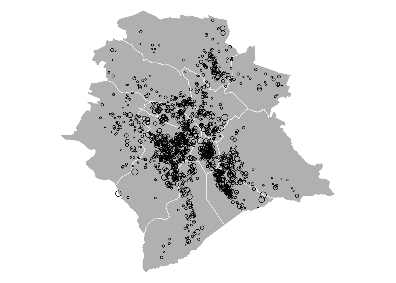
Figure 5.3: Airbnb prices for the Zurich area, 22 June 2017. The size of the circles is proportional to the prices. White lines delineate the 12 districts of the city.
Let us regress prices on the covariates as well as on district dummies:
eq_noFE <- lm(price~bedrooms+accommodates,data=airbnb)
eq_FE   <- lm(price~bedrooms+accommodates+neighborhood,data=airbnb)
# Adjust standard errors:
cov_FE          <- vcovHC(eq_FE, cluster = airbnb[, c("neighborhood")])
robust_se_FE    <- sqrt(diag(cov_FE))
cov_noFE        <- vcovHC(eq_noFE, cluster = airbnb[, c("neighborhood")])
robust_se_noFE  <- sqrt(diag(cov_noFE))
stargazer::stargazer(eq_FE, eq_noFE, eq_FE, eq_noFE, type = "text",
                     column.labels = c("FE (no HAC)", "No FE (no HAC)",
                                       "FE (with HAC)", "No FE (with HAC)"),
                     omit = c("neighborhood"),no.space = TRUE,
                     omit.labels = c("District FE"),keep.stat = "n",
                     se = list(NULL, NULL, robust_se_FE, robust_se_noFE))
##
## ======================================================================
## Dependent variable:
## ---------------------------------------------------------
## price
## FE (no HAC) No FE (no HAC) FE (with HAC) No FE (with HAC)
## (1) (2) (3) (4)
## ----------------------------------------------------------------------
## bedrooms 7.229*** 5.629** 7.229*** 5.629***
## (2.135) (2.194) (2.052) (2.073)
## accommodates 16.426*** 17.449*** 16.426*** 17.449***
## (1.284) (1.323) (1.431) (1.428)
## Constant 95.118*** 68.417*** 95.118*** 68.417***
## (5.323) (3.223) (5.664) (3.527)
## ----------------------------------------------------------------------
## District FE Yes No Yes No
## ----------------------------------------------------------------------
## Observations 1,321 1,321 1,321 1,321
## ======================================================================
## Note: *p<0.1; **p<0.05; ***p<0.01Figure 5.4 compares the residuals with and without fixed effects. The sizes of the circles are proportional to the absolute values of the residuals, the color indicates the sign (blue for positive).
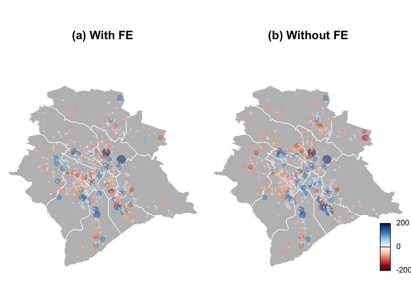
Figure 5.4: Regression residuals. The sizes of the circles are proportional to the absolute values of the residuals, the color indicates the sign (blue for negative).
With fixed effects, the colors are better balanced within each district.
5.5 Dynamic Panel Regressions
In what precedes, it has been assumed that there is no correlation between the observations indexed by \((i,t)\) and those indexed by \((j,s)\) as long as \(j \ne i\) or \(t \ne s\). If one suspects that the errors \(\varepsilon_{i,t}\) are correlated (across entities \(i\) for a given date \(t\), or across dates for a given entity, or both), then one should employ a robust covariance matrix (see Section 4.5.5).
In several cases, auto-correlation in the variable of interest may stem from an auto-regressive specification. That is, Eq. (5.1) is then replaced by: \[\begin{equation} y_{i,t} = \rho y_{i,t-1} + \mathbf{x}'_{i,t}\underbrace{\boldsymbol\beta}_{K \times 1} + \underbrace{\alpha_i}_{\mbox{Individual effects}} + \varepsilon_{i,t}.\tag{5.8} \end{equation}\]
In that case, even if the explanatory variables \(\mathbf{x}_{i,t}\) are uncorrelated to the errors \(\varepsilon_{i,t}\), we have that the additional explanatory variable \(y_{i,t-1}\) correlates to the errors \(\varepsilon_{i,t-1},\varepsilon_{i,t-2},\dots,\varepsilon_{i,1}\). As a result, the LSDV estimate of the model parameters \(\{\rho,\boldsymbol\beta\}\) may be biased, even if \(n\) is large. To see this, notice that the LSDV regression amounts to regressing \(\widetilde{\mathbf{y}}\) on \(\widetilde{\mathbf{X}}\) (see Eq. (5.4)), where the elements of \(\widetilde{\mathbf{X}}\) are the explanatory variables from which we subtract their within-sample means. In particular, we have: \[ \tilde{y}_{i,t-1} = y_{i,t-1} - \frac{1}{T} \sum_{s=1}^{T} y_{i,s-1}, \] which correlates to the corresponding error, that is: \[ \tilde{\varepsilon}_{i,t} = \varepsilon_{i,t} - \frac{1}{T} \sum_{s=1}^{T} \varepsilon_{i,s}. \]
The previous equation shows that the within-group estimator (LSDV) introduces all realizations of the \(\varepsilon_{i,t}\) errors into the transformed error term (\(\tilde{\varepsilon}_{i,t}\)). As a result, in large-\(n\) fixed-\(T\) panels, it is consistent only if all the right-hand-side variables of the regression are strictly exogenous (i.e., do not correlate to past, present, and future errors \(\varepsilon_{i,t}\)).10 This is not the case when there are lags of \(y_{i,t}\) on the right-hand side of the regression formula.
The following simulation illustrate this bias. The \(x\)-coordinates of the dots are the fixed effects \(\alpha_i\)’s, and the \(y\)-coordinates are their LSDV estimates. The blue line is the 45-degree line.
n <- 400;T <- 10
rho <- 0.8;sigma <- .5
alpha <- rnorm(n)
y <- alpha /(1-rho) + sigma^2/(1 - rho^2) * rnorm(n)
all_y <- y
for(t in 2:T){
  y <- rho * y + alpha + sigma * rnorm(n)
  all_y <- rbind(all_y,y)
}
y   <- c(all_y[2:T,]);y_1 <- c(all_y[1:(T-1),])
D <- diag(n) %x% rep(1,T-1)
Z <- cbind(c(y_1),D)
b <- solve(t(Z) %*% Z) %*% t(Z) %*% y
a <- b[2:(n+1)]
plot(alpha,a)
lines(c(-10,10),c(-10,10),col="blue")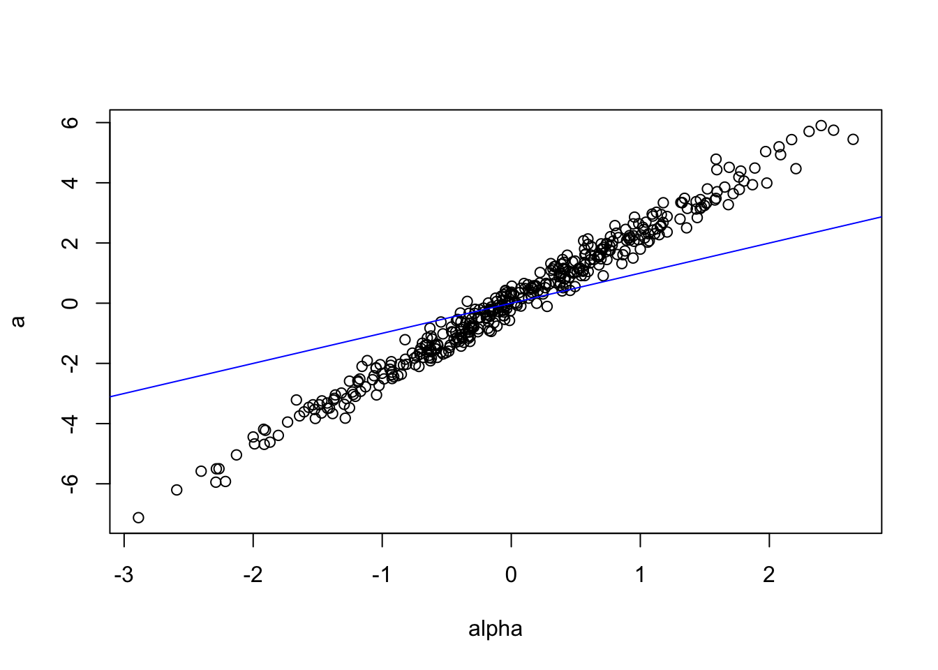
Figure 5.5: illustration of the bias pertianing to the LSDV estimation approach in the presence of auto-correlation of the depend variable.
In the previous example, the estimate of \(\rho\) (whose true value is 0.8) is 0.531.
To address this, one can resort to instrumental-variable regressions. Anderson and Hsiao (1982) have, in particular, proposed a first-differenced Two Stage Least Squares (2SLS) estimator (see Eq. (4.22) in Section 4.4). This estimation is based on the following transformation of the model: \[\begin{equation} \Delta y_{i,t} = \rho \Delta y_{i,t-1} + (\Delta \mathbf{x}_{i,t})'\boldsymbol\beta + \Delta\varepsilon_{i,t}.\tag{5.9} \end{equation}\] The OLS estimates of the parameters are biased because \(\varepsilon_{i,t-1}\) —which is part of the error \(\Delta\varepsilon_{i,t}\)— is correlated to \(y_{i,t-1}\) —which is part of the “explanatory variable”, namely \(\Delta y_{i,t-1}\). But consistent estimates can be obtained using 2SLS with instrumental variables that are correlated with \(\Delta y_{i,t}\) but orthogonal to \(\Delta\varepsilon_{i,t}\). One can for instance use \(\{y_{i,t-2},\mathbf{x}_{i,t-2}\}\) as instruments. Note that this approach can be implemented only if there are more than 3 time observations per entity \(i\).
If the explanatory variables \(\mathbf{x}_{i,t}\) are assumed to be predetermined (i.e., do not contemporaneous correlate with the errors \(\varepsilon_{i,t}\)), then \(\mathbf{x}_{i,t-1}\) can be added to the instruments associated with \(\Delta y_{i,t}\). Further, if these variables (the \(\mathbf{x}_{i,t}\)’s) are exogenous (i.e., do not contemporaneous correlate with any of the errors \(\varepsilon_{i,s}\), \(\forall s\)), then \(\mathbf{x}_{i,t}\) also constitute a valid instrument.
Using the previous (simulated) example, this approach consists in the following steps:
Dy   <- c(all_y[3:T,]) - c(all_y[2:(T-1),])
Dy_1 <- c(all_y[2:(T-1),]) - c(all_y[1:(T-2),])
y_2  <- c(all_y[1:(T-2),])
Z <- matrix(y_2,ncol=1)
Pz <- Z %*% solve(t(Z) %*% Z) %*% t(Z)
Dy_1hat <- Pz %*% Dy_1
rho_2SLS <- solve(t(Dy_1hat) %*% Dy_1hat) %*% t(Dy_1hat) %*% Dy
While the OLS estimate of \(\rho\) (whose true value is 0.8) was 0.531, we obtain here rho_2SLS \(=\) 0.89.
Let us come back to the general case (with covariates \(\mathbf{x}_{i,k}\)’s). For \(t=3\), \(y_{i,1}\) (and \(\mathbf{x}_{i,1}\)) is the only possible instrument. However, for \(t=4\), one could use \(y_{i,2}\) and \(y_{i,1}\) (as well as \(\mathbf{x}_{i,2}\) and \(\mathbf{x}_{i,1}\)). More generally, defining matrix \(Z_i\) as follows: \[ Z_i = \left[ \begin{array}{ccccccccccccccccc} \mathbf{z}_{i,1}' & 0 & \dots \\ 0 & \mathbf{z}_{i,1}' & \mathbf{z}_{i,2}' & 0 & \dots \\ 0 &0 &0 & \mathbf{z}_{i,1} & \mathbf{z}_{i,2}' & \mathbf{z}_{i,3}' & 0 & \dots \\ \vdots \\ 0 & \dots &&&&&& 0 & \mathbf{z}_{i,1}' & \dots & \mathbf{z}_{i,T-2}' \end{array} \right], \] where \(\mathbf{z}_{i,t} = [y_{i,t},\mathbf{x}_{i,t}']'\), we have the moment conditions:11 \[ \mathbb{E}(Z_i'\Delta {\boldsymbol\varepsilon}_i)=0, \]
with \(\Delta{\boldsymbol\varepsilon}_i = [ \Delta \varepsilon_{i,3},\dots,\Delta \varepsilon_{i,T}]'\).
These restrictions are used in the GMM approach employed by Arellano and Bond (1991). Specifically, a GMM estimator of the model parameters is given by: \[ \mbox{argmin}\;\left(\frac{1}{n} \sum_{i=1}^n Z_i' \Delta \boldsymbol\varepsilon_i\right)'W_n\left(\frac{1}{n} \sum_{i=1}^n Z_i' \Delta \boldsymbol\varepsilon_i\right), \] using the weighting matrix \[ W_n = \left(\frac{1}{n}\sum_{i=1}^n Z_i'\widehat{\Delta\boldsymbol\varepsilon_i}\widehat{\Delta\boldsymbol\varepsilon_i}'Z_i\right)^{-1}, \] where the \(\widehat{\Delta\boldsymbol\varepsilon_i}\)’s are consistent estimates of the \(\Delta\boldsymbol\varepsilon_i\)’s that result from a preliminary estimation. In this sense, this estimator is a two-step GMM one.
If the disturbances are homoskedastic, then it can be shown that an asymptotically equivalent (efficient) GMM estimator can be obtained by using: \[ W_{1,n} = \left(\frac{1}{n}Z_i'HZ_i\right)^{-1}, \] where \(H\) is is \((T-2) \times (T-2)\) matrix of the form: \[ H = \left[\begin{array}{ccccccc} 2 & -1 & 0 & \dots &0 \\ -1 & 2 & -1 & & \vdots \\ 0 & \ddots& \ddots & \ddots & 0 \\ \vdots & & -1 & 2&-1\\ 0&\dots & 0 & -1 & 2 \end{array}\right]. \]
It is straightforward to extend these GMM methods to cases where there is more than one lag of the dependent variable on the right-hand side of the equation or in cases where disturbances feature limited moving-average serial correlation.
The pdynmc package allows to run these GMM approaches (see Fritsch, Pua, and Schnurbus (2019)). The following lines of code allow to replicate the results of Arellano and Bond (1991):
library(pdynmc)
data(EmplUK, package = "plm")
dat <- EmplUK
dat[,c(4:7)]         <- log(dat[,c(4:7)])
m1 <- pdynmc(dat = dat, # name of the dataset
             varname.i = "firm", # name of the cross-section identifier
             varname.t = "year", # name of the time-series identifiers
             use.mc.diff = TRUE, # use moment conditions from equations in differences? (i.e. instruments in levels)
             use.mc.lev = FALSE, # use moment conditions from equations in levels? (i.e. instruments in differences)
             use.mc.nonlin = FALSE, # use nonlinear (quadratic) moment conditions?
             include.y = TRUE, # instruments should be derived from the lags of the dependent variable?
             varname.y = "emp", # name of the dependent variable in the dataset
             lagTerms.y = 2, # number of lags of the dependent variable
             fur.con = TRUE, # further control variables (covariates) are included?
             fur.con.diff = TRUE, # include further control variables in equations from differences ?
             fur.con.lev = FALSE, # include further control variables in equations from level?
             varname.reg.fur = c("wage", "capital", "output"), # covariate(s) -in the dataset- to treat as further controls
             lagTerms.reg.fur = c(1,2,2), # number of lags of the further controls
             include.dum = TRUE, # A logical variable indicating whether dummy variables for the time periods are included (defaults to 'FALSE').
             dum.diff = TRUE, # A logical variable indicating whether dummy variables are included in the equations in first differences (defaults to 'NULL').
             dum.lev = FALSE, # A logical variable indicating whether dummy variables are included in the equations in levels (defaults to 'NULL').
             varname.dum = "year",
             w.mat = "iid.err", # One of the character strings c('"iid.err"', '"identity"', '"zero.cov"') indicating the type of weighting matrix to use (defaults to '"iid.err"')
             std.err = "corrected",
             estimation = "onestep", # One of the character strings c('"onestep"', '"twostep"', '"iterative"'). Denotes the number of iterations of the parameter procedure (defaults to '"twostep"').
             opt.meth = "none" # numerical optimization procedure. When no nonlinear moment conditions are employed in estimation, closed form estimates can be computed by setting the argument to '"none"
)
summary(m1,digits=3)
##
## Dynamic linear panel estimation (onestep)
## GMM estimation steps: 1
##
## Coefficients:
## Estimate Std.Err.rob z-value.rob Pr(>|z.rob|)
## L1.emp 0.686226 0.144594 4.746 < 2e-16 ***
## L2.emp -0.085358 0.056016 -1.524 0.12751
## L0.wage -0.607821 0.178205 -3.411 0.00065 ***
## L1.wage 0.392623 0.167993 2.337 0.01944 *
## L0.capital 0.356846 0.059020 6.046 < 2e-16 ***
## L1.capital -0.058001 0.073180 -0.793 0.42778
## L2.capital -0.019948 0.032713 -0.610 0.54186
## L0.output 0.608506 0.172531 3.527 0.00042 ***
## L1.output -0.711164 0.231716 -3.069 0.00215 **
## L2.output 0.105798 0.141202 0.749 0.45386
## 1979 0.009554 0.010290 0.929 0.35289
## 1980 0.022015 0.017710 1.243 0.21387
## 1981 -0.011775 0.029508 -0.399 0.68989
## 1982 -0.027059 0.029275 -0.924 0.35549
## 1983 -0.021321 0.030460 -0.700 0.48393
## 1976 -0.007703 0.031411 -0.245 0.80646
## ---
## Signif. codes: 0 '***' 0.001 '**' 0.01 '*' 0.05 '.' 0.1 ' ' 1
##
## 41 total instruments are employed to estimate 16 parameters
## 27 linear (DIF)
## 8 further controls (DIF)
## 6 time dummies (DIF)
##
## J-Test (overid restrictions): 70.82 with 25 DF, pvalue: <0.001
## F-Statistic (slope coeff): 528.06 with 10 DF, pvalue: <0.001
## F-Statistic (time dummies): 14.98 with 6 DF, pvalue: 0.0204We generate novel results (m2) by replacing “onestep” with “twostep” (in the estimation field). The resulting estimated coefficients are:
##      L1.emp      L2.emp     L0.wage     L1.wage  L0.capital  L1.capital
##  0.62870890 -0.06518800 -0.52575951  0.31128961  0.27836190  0.01409950
##  L2.capital   L0.output   L1.output   L2.output        1979        1980
## -0.04024847  0.59192286 -0.56598515  0.10054264  0.01121551  0.02306871
##        1981        1982        1983        1976
## -0.02135806 -0.03111604 -0.01799335 -0.02336762
Arellano and Bond (1991) have proposed a specification test. If the model is correctly specified, then the errors of Eq. (5.9) —that is the first-difference equation— should feature non-zero first-order auto-correlations, but zero higher-order autocorrelations.
Function mtest.fct of package pdynmc implements this test. Here is its result in the present case:
mtest.fct(m1,order=3)##
## Arellano and Bond (1991) serial correlation test of degree 3
##
## data: 1step GMM Estimation
## normal = 0.045945, p-value = 0.9634
## alternative hypothesis: serial correlation of order 3 in the error termsOne can also implement the Hansen J-test of the over-identifying restrictions (see Section 6.1.3):
jtest.fct(m1)##
## J-Test of Hansen
##
## data: 1step GMM Estimation
## chisq = 70.82, df = 25, p-value = 2.905e-06
## alternative hypothesis: overidentifying restrictions invalid
jtest.fct(m2)##
## J-Test of Hansen
##
## data: 2step GMM Estimation
## chisq = 31.381, df = 25, p-value = 0.1767
## alternative hypothesis: overidentifying restrictions invalid5.6 Introduction to program evaluation
This section brielfy introduces the econometrics of program evaluation. Program evaluation refer to the analysis of the causal effects of some “treatments” in a broad sense. These treatment can, e.g., correspond to the implementation (or announcement) of policy measures. A comprehensive review is proposed by Abadie and Cattaneo (2018). A seminal book on the subject is that of Angrist and Pischke (2008).
5.6.1 Presentation of the problem
To begin with, let us consider a single entity. To simplify notations, we drop the entity index (\(i\)). Let us denote by \(Y\) the outcome variable (for the variable of interest), by \(W\) is a binary variable indicating whether the considered entity has received treatment (\(W=1\)) or not (\(W=0\)), and by \(X\) a vector of covariates, assumed to be predetermined relative to the treatment. That is, \(W\) and \(X\) could be correlated, but the values of \(X\) have been determined before that of \(W\) (in such a way that the realization of \(W\) does not affect \(X\)). Typcally, \(X\) contains characteristics of the considered entity.
We are interested in the effect of the treatment, that is: \[ Y_1 - Y_0, \] where \(Y_1\) correspond to the outcome obtained under treatment, while \(Y_0\) is the outcome obtained without it. Notice that we have: \[ Y = (1-W) Y_0 + W Y_1. \]
The problem is that observing \((Y,W,X)\) is not sufficient to observe the treatment effect \(Y_1 - Y_0\). Additional assumptions are needed to estimate it, or, more precisely, its expectations (average treatment effect): \[ ATE = \mathbb{E}(Y_1 - Y_0). \]
Importantly, \(ATE\) is different from the following quantity: \[ \alpha = \underbrace{\mathbb{E}(Y|W=1)}_{=\mathbb{E}(Y_1|W=1)} - \underbrace{\mathbb{E}(Y|W=0)}_{=\mathbb{E}(Y_0|W=0)}, \] that is easier to estimate. Indeed, a consistent estimate of \(\alpha\) is the difference between the means of the outcome variables in two sub-samples: one containing only the treated entities (this gives an estimate of \(\mathbb{E}(Y_1|W=1)\)) and the other containing only the non-treated entities (this gives an estimate of \(\mathbb{E}(Y_0|W=0)\)). Coming back to \(ATE\), the problem is that we won’t have direct information regarding \(\mathbb{E}(Y_0|W=1)\) and \(\mathbb{E}(Y_1|W=0)\). However, these two conditional expectations are part of \(ATE\). Indeed, \(ATE = \mathbb{E}(Y_1) - \mathbb{E}(Y_0)\), and: \[\begin{eqnarray} \mathbb{E}(Y_1) &=& \mathbb{E}(Y_1|W=0)\mathbb{P}(W=0)+\mathbb{E}(Y_1|W=1)\mathbb{P}(W=1) \tag{5.10} \\ \mathbb{E}(Y_0) &=& \mathbb{E}(Y_0|W=0)\mathbb{P}(W=0)+\mathbb{E}(Y_0|W=1)\mathbb{P}(W=1). \tag{5.11} \end{eqnarray}\]
5.6.2 Randomized controlled trials (RCTs)
In the context of Randomized controlled trials (RCTs), entities are randomly assigned to receive the treatment. As a result, we have \(\mathbb{E}(Y_1) = \mathbb{E}(Y_1|W=0) = \mathbb{E}(Y_1|W=1)\) and \(\mathbb{E}(Y_0) = \mathbb{E}(Y_0|W=0) = \mathbb{E}(Y_0|W=1)\). Using this into Eqs. (5.10) and (5.11) yields \(ATE = \alpha\).
Therefore, in this context, estimating \(\mathbb{E}(Y_1-Y_0)\) amounts to computing the difference between two sample means, namely (a) the sample mean of the subset of \(Y_i\)’s corresponding to the entities for which \(W_i=1\), and (b) the one for which \(W_i=0\).
More accurate estimates can be obtained through regressions. Assume that the model reads: \[ Y_{i} = W_{i} \beta_{1} + X_i'\boldsymbol\beta_z + \varepsilon_i, \] where \(\mathbb{E}(\varepsilon_i|X_i) = 0\) (and \(W_i\) is independent from \(X_i\) and \(\varepsilon_i\)). In this case, we obtain a consistent estimate of \(\beta_1\) by regressing \(\mathbf{y}\) on \(\mathbf{Z} = [\mathbf{w},\mathbf{X}]\).
5.6.3 Difference-in-Difference (DiD) approach
The DiD approach is a popular methodology implemented in cases where \(W\) cannot be considered as an independent variable. It exploits two dimensions: entities (\(i\)), and time (\(t\)). To simplify the exposition, we consider only two periods here (\(t=0\) and \(t=1\)).
Consider the following model: \[\begin{equation} Y_{i,t} = W_{i,t} \beta_1 + \mu_i + \delta_t + \varepsilon_{i,t}\tag{5.12} \end{equation}\]
The parameter of interest is \(\beta_{1}\), which is the treatment effect (recall that \(W_{i,t} \in \{0,1\}\)). Usually, for all entities \(i\), we have \(W_{i,t=0}=0\). But only some of them are treated on date 1, i.e., \(W_{i,1} \in \{0,1\}\).
The disturbance \(\varepsilon_{i,t}\) affects the outcome, but we assume that it does not relate to the selection for treatment; therefore, \(\mathbb{E}(\varepsilon_{i,t}|W_{i,t})=0\). By contrast, we do not exclude some correlation between \(W_{i,t}\) (for \(t=1\)) and \(\mu_i\); hence, \(\mu_i\) may constitute a confounder. Finally, we suppose that the micro-variables \(W_i\) do not affect the time fixed effects \(\delta_t\), such that \(\mathbb{E}(\delta_t|W_{i,t})=\mathbb{E}(\delta_t)\).
We have:
\[ \begin{array}{cccccccccc} \mathbb{E}(Y_{i,1}|W_{i,1}=1) &=& \beta_1 &+& \mathbb{E}(\mu_i|W_{i,1}=1) &+&\mathbb{E}(\delta_1|W_{i,1}=1) &+& \mathbb{E}(\varepsilon_{i,1}) \\ \mathbb{E}(Y_{i,0}|W_{i,1}=1) &=& && \mathbb{E}(\mu_i|W_{i,1}=1) &+&\mathbb{E}(\delta_0|W_{i,1}=1) &+& \mathbb{E}(\varepsilon_{i,0}) \\ \mathbb{E}(Y_{i,1}|W_{i,1}=0) &=& && \mathbb{E}(\mu_i|W_{i,1}=0) &+&\mathbb{E}(\delta_1|W_{i,1}=0) &+& \mathbb{E}(\varepsilon_{i,1}) \\ \mathbb{E}(Y_{i,0}|W_{i,1}=0) &=& && \mathbb{E}(\mu_i|W_{i,1}=0) &+&\mathbb{E}(\delta_0|W_{i,1}=0) &+& \mathbb{E}(\varepsilon_{i,0}). \end{array} \] and, under our assumptions, it can be checked that:
\[ \beta_1 = \mathbb{E}(\Delta Y_{i,1}|W_{i,1}=1) - \mathbb{E}(\Delta Y_{i,1}|W_{i,1}=0), \] where \(\Delta Y_{i,1}=Y_{i,1}-Y_{i,0}\). Therefore, in this context, the treatment effect appears to be a difference (of two conditionnal expectations) of difference (of the outcome variable, through time).
This is illustrated by Figure 5.6, which represents the generic DiD framework.
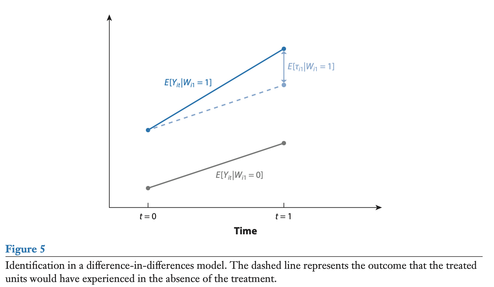
Figure 5.6: Source: Abadie et al., (1998).
In practice, implementing this approach consists in running a linear regression of the type of Eq. (5.12). These regressions often use time-invariant characteristics as controls instead of the ixed effects \(\mu_i\). As illustrated in the next subsection, the parameter of interest (\(\beta_1\)) is often associated with an interaction term.
5.6.4 Application of the DiD approach
This example is based on the data used in Meyer, Viscusi, and Durbin (1995). This dataset is part of the wooldridge package. This paper examines the effect of workers’ compensation for injury on time out of work. It exploits a natural experiment approach of comparing individuals injured before and after increases in the maximum weekly benefit amount. Specifically, in 1980, the cap on weekly earnings covered by worker’s compensation was increased in Kentucky and Michigan. This can be exploited to check whether this new policy was followed by an increase in the amount of time workers spent unemployed (for example, higher compensation may reduce workers’ incentives to avoid injury).
As shown in Figure 5.7, the measure has only affected high-earning workers. The idea exploited by Meyer, Viscusi, and Durbin (1995) was to compare the increase in time out of work before-after 1980 for higher-earnings workers on the one hand (entities who received the treatment) and low-earnings workers on the other hand (control group).
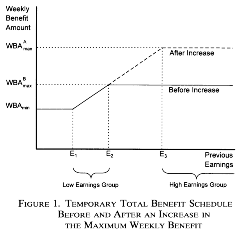
Figure 5.7: Source: Meyer et al., (1995).
The next lines of codes replicate some of their results. The dependent variable is the logarithm of the duration of benefits. For more information use ?injury, after having loaded the wooldridge library.
In the table of results below, the parameter of interest is the one associated with the interaction term afchnge:highearn. Columns 2 and 3 correspond to the first two column of Table 6 in Meyer, Viscusi, and Durbin (1995).
library(wooldridge)
data(injury)
injury <- subset(injury,ky==1)
injury$indust <- as.factor(injury$indust)
injury$injtype <- as.factor(injury$injtype)
#names(injury)
eq1 <- lm(log(durat) ~ afchnge + highearn + afchnge*highearn,data=injury)
eq2 <- lm(log(durat) ~ afchnge + highearn + afchnge*highearn +
            lprewage*highearn + male + married + lage + ltotmed + hosp +
            indust + injtype,data=injury)
eq3 <- lm(log(durat) ~ afchnge + highearn + afchnge*highearn +
            lprewage*highearn + male + married + lage + indust +
            injtype,data=injury)
stargazer::stargazer(eq1,eq2,eq3,type="text",
                     omit=c("indust","injtype","Constant"),no.space = TRUE,
                     add.lines = list(c("industry dummy","no","yes","yes"),
                                      c("injury dummy","no","yes","yes")),
                     order = c(1,2,18,3:17,19,20),omit.stat = c("f","ser"))
##
## ===============================================
## Dependent variable:
## -----------------------------
## log(durat)
## (1) (2) (3)
## -----------------------------------------------
## afchnge 0.008 -0.004 0.016
## (0.045) (0.038) (0.045)
## highearn 0.256*** -0.595 -1.522
## (0.047) (0.930) (1.099)
## afchnge:highearn 0.191*** 0.162*** 0.215***
## (0.069) (0.059) (0.069)
## lprewage 0.207** 0.258**
## (0.088) (0.104)
## male -0.070* -0.072
## (0.039) (0.046)
## married 0.055 0.051
## (0.035) (0.041)
## lage 0.244*** 0.252***
## (0.044) (0.052)
## ltotmed 0.361***
## (0.011)
## hosp 0.252***
## (0.044)
## highearn:lprewage 0.065 0.232
## (0.158) (0.187)
## -----------------------------------------------
## industry dummy no yes yes
## injury dummy no yes yes
## Observations 5,626 5,347 5,347
## R2 0.021 0.319 0.049
## Adjusted R2 0.020 0.316 0.046
## ===============================================
## Note: *p<0.1; **p<0.05; ***p<0.01