7 Binary-choice models
In microeconometric models, the variables of interest often feature restricted distributions —for instance with discontinuous support—, which necessitates specific models. Typically, in many instances, the variables to be explained (the \(y_i\)’s) have only two possible values (\(0\) and \(1\), say). That is, they are binary variables. The probability for them to be equal to either 0 or 1 may depend on independent variables, gathered in vectors \(\mathbf{x}_i\) (\(K \times 1\)).
The spectrum of applications is wide:
- Binary decisions (e.g. in referendums, being owner or renter, living in the city or in the countryside, in/out of the labour force,…),
- Contamination (disease or default),
- Success/failure (exams).
Without loss of generality, the model reads: \[\begin{equation}\label{eq:binaryBenroulli} y_i | \mathbf{X} \sim \mathcal{B}(g(\mathbf{x}_i;\boldsymbol\theta)), \end{equation}\] where \(g(\mathbf{x}_i;\boldsymbol\theta)\) is the parameter of the Bernoulli distribution. In other words, conditionally on \(\mathbf{X}\): \[\begin{equation} y_i = \left\{ \begin{array}{cl} 1 & \mbox{ with probability } g(\mathbf{x}_i;\boldsymbol\theta)\\ 0 & \mbox{ with probability } 1-g(\mathbf{x}_i;\boldsymbol\theta), \end{array} \right.\tag{7.1} \end{equation}\] where \(\boldsymbol\theta\) is a vector of parameters to be estimated.
An estimation strategy is to assume that \(g(\mathbf{x}_i;\boldsymbol\theta)\) can be proxied by \(\tilde{\boldsymbol\theta}'\mathbf{x}_i\) and to run a linear regression to estimate \(\tilde{\boldsymbol\theta}\) (a situation called Linear Probability Model, LPM): \[ y_i = \tilde{\boldsymbol\theta}'\mathbf{x}_i + \varepsilon_i. \] Notwithstanding the fact that this specification does not exclude negative probabilities or probabilities greater than one, it could be compatible with the assumption of zero conditional mean (Hypothesis 4.2) and with the assumption of non-correlated residuals (Hypothesis 4.4), but more difficultly with the homoskedasticity assumption (Hypothesis 4.3). Moreover, the \(\varepsilon_i\)’s cannot be Gaussian (because \(y_i \in \{0,1\}\)). Hence, using a linear regression to study the relationship between \(\mathbf{x}_i\) and \(y_i\) can be consistent but it is inefficient.
Figure 7.1 illustrates the fit resulting from an application of the LPM model to binary (dependent) variables.
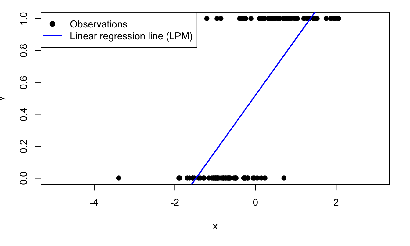
Figure 7.1: Fitting a binary variable with a linear model (Linear Probability Model, LPM). The model is \(\mathbb{P}(y_i=1|x_i)=\Phi(0.5+2x_i)\), where \(\Phi\) is the c.d.f. of the normal distribution and where \(x_i \sim \,i.i.d.\,\mathcal{N}(0,1)\).
Except for its last row (LPM case), Table 7.1 provides examples of functions \(g\) valued in \([0,1]\), and that can therefore used in models of the type: \(\mathbb{P}(y_i=1|\mathbf{x}_i;\boldsymbol\theta) = g(\boldsymbol\theta'\mathbf{x}_i)\) (see Eq. (7.1)). The “linear” case is given for comparison, but note that it does not satisfy \(g(\boldsymbol\theta'\mathbf{x}_i) \in [0,1]\) for any value of \(\boldsymbol\theta'\mathbf{x}_i\).
| Model | Function \(g\) | Derivative |
|---|---|---|
| Probit | \(\Phi\) | \(\phi\) |
| Logit | \(\dfrac{\exp(x)}{1+\exp(x)}\) | \(\dfrac{\exp(x)}{(1+\exp(x))^2}\) |
| log-log | \(1 - \exp(-\exp(x))\) | \(\exp(-\exp(x))\exp(x)\) |
| linear (LPM) | \(x\) | 1 |
Figure 7.2 displays the first three \(g\) functions appearing in Table 7.1.
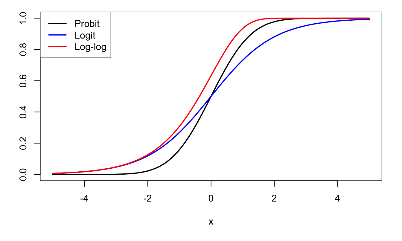
Figure 7.2: Probit, Logit, and Log-log functions.
The probit and the logit models are popular binary-choice models. In the probit model, we have: \[\begin{equation} g(z) = \Phi(z),\tag{7.2} \end{equation}\] where \(\Phi\) is the c.d.f. of the normal distribution. And for the logit model: \[\begin{equation} g(z) = \frac{1}{1+\exp(-z)}.\tag{7.3} \end{equation}\]
Figure 7.3 shows the conditional probabilities associated with the (probit) model that had been used to generate the data of Figure 7.1.
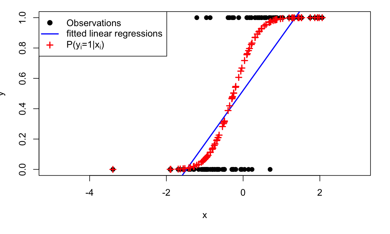
Figure 7.3: The model is \(\mathbb{P}(y_i=1|x_i)=\Phi(0.5+2x_i)\), where \(\Phi\) is the c.d.f. of the normal distribution and where \(x_i \sim \,i.i.d.\,\mathcal{N}(0,1)\). Crosses give the model-implied probabilities of having \(y_i=1\) (conditional on \(x_i\)).
7.1 Interpretation in terms of latent variable, and utility-based models
The probit model has an interpretation in terms of latent variables, which, in turn, is often exploited in structural models, called Random Utility Models (RUM). In such structural models, it is assumed that the agents that have to take the decision do so by selecting the outcome that provides them with the larger utility (for agent \(i\), two possible outcomes: \(y_i=0\) or \(y_i=1\)). Part of this utility is observed by the econometrician —it depends on the covariates \(\mathbf{x}_i\)— and part of it is latent.
In the probit model, we have: \[ \mathbb{P}(y_i=1|\mathbf{x}_i;\boldsymbol\theta) = \Phi(\boldsymbol\theta'\mathbf{x}_i) = \mathbb{P}(-\varepsilon_{i}<\boldsymbol\theta'\mathbf{x}_i), \] where \(\varepsilon_{i} \sim \mathcal{N}(0,1)\). That is: \[ \mathbb{P}(y_i=1|\mathbf{x}_i;\boldsymbol\theta) = \mathbb{P}(0< y_i^*), \] where \(y_i^* = \boldsymbol\theta'\mathbf{x}_i + \varepsilon_i\), with \(\varepsilon_{i} \sim \mathcal{N}(0,1)\). Variable \(y_i^*\) can be interpreted as a (latent) variable that determines \(y_i\) (since \(y_i = \mathbb{I}_{\{y_i^*>0\}}\)).
Figure 7.4 illustrates this situation.
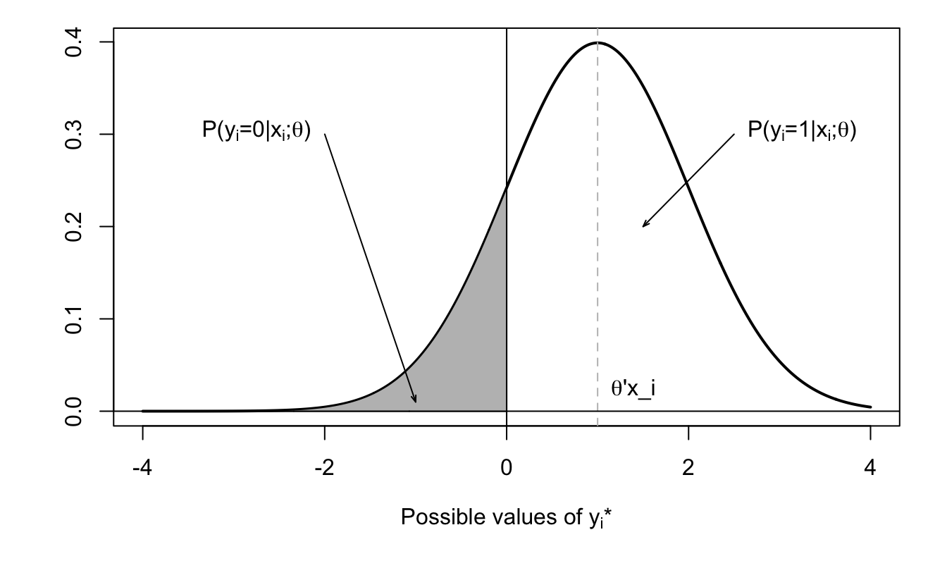
Figure 7.4: Distribution of \(y_i^*\) conditional on \(\mathbf{x}_i\).
Assume that agent (\(i\)) chooses \(y_i=1\) if the utility associated with this choice (\(U_{i,1}\)) is higher than the one associated with \(y_i=0\) (that is \(U_{i,0}\)). Assume further that the utility of agent \(i\), if she chooses outcome \(j\) (\(\in \{0,1\}\)), is given by \[ U_{i,j} = V_{i,j} + \varepsilon_{i,j}, \] where \(V_{i,j}\) is the deterministic component of the utility associated with choice and where \(\varepsilon_{i,j}\) is a random (agent-specific) component. Moreover, posit \(V_{i,j} = \boldsymbol\theta_j'\mathbf{x}_i\). We then have: \[\begin{eqnarray} \mathbb{P}(y_i = 1|\mathbf{x}_i;\boldsymbol\theta) &=& \mathbb{P}(\boldsymbol\theta_1'\mathbf{x}_i+\varepsilon_{i,1}>\boldsymbol\theta_0'\mathbf{x}_i+\varepsilon_{i,0}) \nonumber\\ &=& F(\boldsymbol\theta_1'\mathbf{x}_i-\boldsymbol\theta_0'\mathbf{x}_i) = F([\boldsymbol\theta_1-\boldsymbol\theta_0]'\mathbf{x}_i),\tag{7.4} \end{eqnarray}\] where \(F\) is the c.d.f. of \(\varepsilon_{i,0}-\varepsilon_{i,1}\).
Note that only the difference \(\boldsymbol\theta_1-\boldsymbol\theta_0\) is identifiable (as opposed to \(\boldsymbol\theta_1\) and \(\boldsymbol\theta_0\)). Moreover, replacing \(U\) with \(aU\) (\(a>0\)) gives the same model; this scaling issue can be solved by fixing the variance of \(\varepsilon_{i,0}-\varepsilon_{i,1}\).
Example 7.1 (Migration and income) The RUM approach has been used by Nakosteen and Zimmer (1980) to study migration choices. Their model is based on the comparison of marginal costs and benefits associated with migration. The main ingredients of their approach are as follows:
- Wage that can be earned at the present location: \(y_p^* = \boldsymbol\theta_p'\mathbf{x}_p + \varepsilon_p\).
- Migration cost: \(C^*= \boldsymbol\theta_c'\mathbf{x}_c + \varepsilon_c\).
- Wage earned elsewhere: \(y_m^* = \boldsymbol\theta_m'\mathbf{x}_m + \varepsilon_m\).
In this context, agents decision to migrate if \(y_m^* > y_p^* + C^*\), i.e. if \[ y^* = y_m^* - y_p^* - C^* = \boldsymbol\theta'\mathbf{x} + \underbrace{\varepsilon}_{=\varepsilon_m - \varepsilon_c - \varepsilon_p}>0, \] where \(\mathbf{x}\) is the union of the \(\mathbf{x}_i\)s, for \(i \in \{p,m,c\}\).
7.2 Alternative-Varying Regressors
In some cases, regressors may depend on the considered alternative (\(0\) or \(1\)). For instance:
- When modeling the decision to participate in the labour force (or not), the wage depends on the alternative. Typically, it is zero if the considered agent has decided not to work (and strictly positive otherwise).
- In the context of the choice of transportation mode, “time cost” depends on the considered transportation mode.
In terms of utility, we then have: \[ V_{i,j} = {\theta^{(u)}_{j}}'\mathbf{u}_{i,j} + {\theta^{(v)}_{j}}'\mathbf{v}_{i}, \] where the \(\mathbf{u}_{i,j}\)’s are regressors associated with agent \(i\), but taking different values for the different choices (\(j=0\) or \(j=1\)). In that case, Eq. (7.4) becomes: \[\begin{equation} \mathbb{P}(y_i = 1|\mathbf{x}_i;\boldsymbol\theta) = F\left({\theta^{(u)}_{1}}'\mathbf{u}_{i,1}-{\theta^{(u)}_{0}}'\mathbf{u}_{i,0}+[\boldsymbol\theta_1^{(v)}-\boldsymbol\theta_0^{(v)}]'\mathbf{v}_i\right),\tag{7.5} \end{equation}\] and, if \(\theta^{(u)}_{1}=\theta^{(u)}_{0}=\theta^{(u)}\) —as is customary— we get: \[\begin{equation} \mathbb{P}(y_i = 1|\mathbf{x}_i;\boldsymbol\theta) = F\left({\theta^{(u)}_{1}}'(\mathbf{u}_{i,1}-\mathbf{u}_{i,0})+[\boldsymbol\theta_1^{(v)}-\boldsymbol\theta_0^{(v)}]'\mathbf{v}_i\right).\tag{7.6} \end{equation}\]
Example 7.2 (Fishing-mode dataset) The fishing-mode dataset used in Cameron and Trivedi (2005) (Chapters 14 and 15) contains alternative-specific variables. Specifically, for each individual, the price and catch rate depend on the fishing model. In the table reported below, lines price and catch correspond to the prices and catch rates associated with the chosen alternative.
##
## ==========================================================
## Statistic       N     Mean    St. Dev.    Min      Max
## ----------------------------------------------------------
## price.beach   1,182  103.422   103.641   1.290   843.186
## price.pier    1,182  103.422   103.641   1.290   843.186
## price.boat    1,182  55.257    62.713    2.290   666.110
## price.charter 1,182  84.379    63.545   27.290   691.110
## catch.beach   1,182   0.241     0.191    0.068    0.533
## catch.pier    1,182   0.162     0.160    0.001    0.452
## catch.boat    1,182   0.171     0.210   0.0002    0.737
## catch.charter 1,182   0.629     0.706    0.002    2.310
## income        1,182 4,099.337 2,461.964 416.667 12,500.000
## ----------------------------------------------------------
7.3 Estimation
These models can be estimated by Maximum Likelihood approaches (see Section 6.2).
To simplify the exposition, we consider the \(\mathbf{x}_i\) vectors of covariates to be deterministic. Moreover, we assume that the r.v. are independent across entities \(i\). How to write the likelihood in that case? It is easily checked that: \[ f(y_i|\mathbf{x}_i;\boldsymbol\theta) = g(\boldsymbol\theta'\mathbf{x}_i)^{y_i}(1-g(\boldsymbol\theta'\mathbf{x}_i))^{1-y_i}. \]
Therefore, if the observations \((\mathbf{x}_i,y_i)\) are independent across entities \(i\), we obtain: \[ \log \mathcal{L}(\boldsymbol\theta;\mathbf{y},\mathbf{X}) = \sum_{i=1}^{n}y_i \log[g(\boldsymbol\theta'\mathbf{x}_i)] + (1-y_i)\log[1-g(\boldsymbol\theta'\mathbf{x}_i)]. \]
The likelihood equation reads (FOC of the optimization program, see Def. 6.7): \[ \dfrac{\partial \log \mathcal{L}(\boldsymbol\theta;\mathbf{y},\mathbf{X})}{\partial \boldsymbol\theta} = \mathbf{0}, \] that is: \[ \sum_{i=1}^{n} y_i \mathbf{x}_i\frac{g'(\boldsymbol\theta'\mathbf{x}_i)}{g(\boldsymbol\theta'\mathbf{x}_i)} - (1-y_i) \mathbf{x}_i \frac{g'(\boldsymbol\theta'\mathbf{x}_i)}{1-g(\boldsymbol\theta'\mathbf{x}_i)} = \mathbf{0}. \]
This is a nonlinear (multivariate) equation that can be solved numerically. Under regularity conditions (Hypotheses 6.1), we approximately have (Prop. 6.4): \[ \boldsymbol\theta_{MLE} \sim \mathcal{N}(\boldsymbol\theta_0,\mathbf{I}(\boldsymbol\theta_0)^{-1}), \] where \[ \mathbf{I}(\boldsymbol\theta_0) = - \mathbb{E}_0 \left( \frac{\partial^2 \log \mathcal{L}(\theta;\mathbf{y},\mathbf{X})}{\partial \boldsymbol\theta \partial \boldsymbol\theta'}\right) = n \mathcal{I}_Y(\boldsymbol\theta_0). \]
For finite samples, we can e.g. approximate \(\mathbf{I}(\boldsymbol\theta_0)^{-1}\) by Eq. (6.10): \[ \mathbf{I}(\boldsymbol\theta_0)^{-1} \approx -\left(\frac{\partial^2 \log \mathcal{L}(\boldsymbol\theta_{MLE};\mathbf{y},\mathbf{X})}{\partial \boldsymbol\theta \partial \boldsymbol\theta'}\right)^{-1}. \]
In the Probit case (see Table 7.1), it can be shown that we have: \[\begin{eqnarray*} &&\frac{\partial^2 \log \mathcal{L}(\boldsymbol\theta;\mathbf{y},\mathbf{X})}{\partial \boldsymbol\theta \partial \boldsymbol\theta'} = - \sum_{i=1}^{n} g'(\boldsymbol\theta'\mathbf{x}_i) [\mathbf{x}_i \mathbf{x}_i'] \times \\ &&\left[y_i \frac{g'(\boldsymbol\theta'\mathbf{x}_i) + \boldsymbol\theta'\mathbf{x}_ig(\boldsymbol\theta'\mathbf{x}_i)}{g(\boldsymbol\theta'\mathbf{x}_i)^2} + (1-y_i) \frac{g'(\boldsymbol\theta'\mathbf{x}_i) - \boldsymbol\theta'\mathbf{x}_i (1 - g(\boldsymbol\theta'\mathbf{x}_i))}{(1-g(\boldsymbol\theta'\mathbf{x}_i))^2}\right]. \end{eqnarray*}\]
In the Logit case (see Table 7.1), it can be shown that we have: \[ \frac{\partial^2 \log \mathcal{L}(\boldsymbol\theta;\mathbf{y},\mathbf{X})}{\partial \boldsymbol\theta \partial \boldsymbol\theta'} = - \sum_{i=1}^{n} g'(\boldsymbol\theta'\mathbf{x}_i) \mathbf{x}_i\mathbf{x}_i', \] where \(g'(x)=\dfrac{\exp(-x)}{(1 + \exp(-x))^2}\).
Remark that, since \(g'(x)>0\), \(-\partial^2 \log \mathcal{L}(\boldsymbol\theta;\mathbf{y},\mathbf{X})/\partial \boldsymbol\theta \partial \boldsymbol\theta'\) is positive definite.
7.4 Marginal effects
How to measure marginal effects, i.e. the effect on the probability that \(y_i=1\) of a marginal increase of \(x_{i,k}\)? This object is given by: \[ \frac{\partial \mathbb{P}(y_i=1|\mathbf{x}_i;\boldsymbol\theta)}{\partial x_{i,k}} = \underbrace{g'(\boldsymbol\theta'\mathbf{x}_i)}_{>0}\theta_k, \] which is of the same sign as \(\theta_k\) if function \(g\) is monotonously increasing.
For agent \(i\), this marginal effect is consistently estimated by \(g'(\boldsymbol\theta_{MLE}'\mathbf{x}_i)\theta_{MLE,k}\). It is important to see that the marginal effect depends on \(\mathbf{x}_i\): respective increases by 1 unit of \(x_{i,k}\) (entity \(i\)) and of \(x_{j,k}\) (entity \(j\)) do not necessarily have the same effect on \(\mathbb{P}(y_i=1|\mathbf{x}_i;\boldsymbol\theta)\) as on \(\mathbb{P}(y_j=1|\mathbf{x}_j;\boldsymbol\theta)\). To address this issue, one can compute some measures of “average” marginal effect. There are two main solutions. For each explanatory variable \(k\):
- Denoting by \(\hat{\mathbf{x}}\) the sample average of the \(\mathbf{x}_i\)s, compute \(g'(\boldsymbol\theta_{MLE}'\hat{\mathbf{x}})\theta_{MLE,k}\).
- Compute the average (across \(i\)) of \(g'(\boldsymbol\theta_{MLE}'\mathbf{x}_i)\theta_{MLE,k}\).
7.5 Goodness of fit
There is no obvious version of “\(R^2\)” for binary-choice models. Existing measures are called pseudo-\(R^2\) measures.
Denoting by \(\log \mathcal{L}_0(\mathbf{y})\) the (maximum) log-likelihood that would be obtained for a model containing only a constant term (i.e. with \(\mathbf{x}_i = 1\) for all \(i\)), the McFadden’s pseudo-\(R^2\) is given by: \[ R^2_{MF} = 1 - \frac{\log \mathcal{L}(\boldsymbol\theta;\mathbf{y})}{\log \mathcal{L}_0(\mathbf{y})}. \] Intuitively, \(R^2_{MF}=0\) if the explanatory variables do not convey any information on the outcome \(y\). Indeed, in this case, the model is not better than the reference model, that simply captures the fraction of \(y_i\)’s that are equal to 1.
Example 7.3 (Credit and defaults (Lending-club dataset)) This example makes use of the credit data of package AEC. The objective is to model the default probabilities of borrowers.
Let us first represent the relationship between the fraction of households that have defaulted on their loan and their annual income:
library(AEC)
credit$Default <- 0
credit$Default[credit$loan_status == "Charged Off"] <- 1
credit$Default[credit$loan_status ==
                 "Does not meet the credit policy. Status:Charged Off"] <- 1
credit$amt2income <- credit$loan_amnt/credit$annual_inc
plot(as.factor(credit$Default)~log(credit$annual_inc),
     ylevels=2:1,ylab="Default status",xlab="log(annual income)")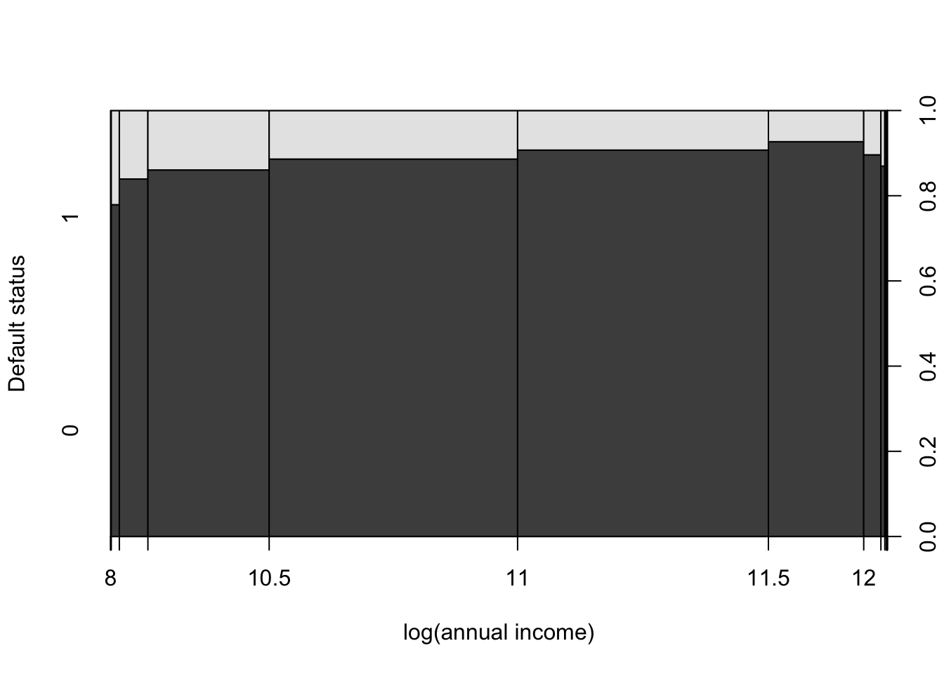
The previous figure suggests that the effect of annual income on the probability of default is non-monotonous. We will therefore include a quadratic term in one of our specification (namely eq1 below).
We consider three specifications. The first one (eq0), with no explanatory variables, is trivial. It will just be used to compute the pseudo-\(R^2\). In the second (eq1), we consider a few covariates (loan amount, the ratio between the amount and annual income, The number of more-than-30 days past-due incidences of delinquency in the borrower’s credit file for the past 2 years, and a quadratic function of annual income). In the third model (eq2), we add a credit rating.
eq0 <- glm(Default ~ 1,data=credit,family=binomial(link="probit"))
eq1 <- glm(Default ~ log(loan_amnt) + amt2income + delinq_2yrs +
             log(annual_inc)+ I(log(annual_inc)^2),
           data=credit,family=binomial(link="probit"))
eq2 <- glm(Default ~ grade + log(loan_amnt) + amt2income + delinq_2yrs +
             log(annual_inc)+ I(log(annual_inc)^2),
           data=credit,family=binomial(link="probit"))
stargazer::stargazer(eq0,eq1,eq2,type="text",no.space = TRUE)
##
## ====================================================
## Dependent variable:
## --------------------------------
## Default
## (1) (2) (3)
## ----------------------------------------------------
## gradeB 0.399***
## (0.055)
## gradeC 0.588***
## (0.057)
## gradeD 0.820***
## (0.061)
## gradeE 0.857***
## (0.092)
## gradeF 1.243***
## (0.148)
## gradeG 1.439***
## (0.227)
## log(loan_amnt) -0.150** -0.194***
## (0.060) (0.061)
## amt2income 1.281*** 1.227***
## (0.384) (0.393)
## delinq_2yrs 0.097*** 0.010
## (0.034) (0.035)
## log(annual_inc) -1.464** -0.933
## (0.573) (0.589)
## I(log(annual_inc)2) 0.065*** 0.041
## (0.025) (0.026)
## Constant -1.232*** 8.035*** 5.078
## (0.017) (3.084) (3.172)
## ----------------------------------------------------
## Observations 9,136 9,136 9,136
## Log Likelihood -3,144.885 -3,107.976 -2,969.893
## Akaike Inf. Crit. 6,291.769 6,227.953 5,963.787
## ====================================================
## Note: *p<0.1; **p<0.05; ***p<0.01Let us compute the pseudo R2 for the last two models:
logL0 <- logLik(eq0);logL1 <- logLik(eq1);logL2 <- logLik(eq2)
pseudoR2_eq1 <- 1 - logL1/logL0 # pseudo R2
pseudoR2_eq2 <- 1 - logL2/logL0 # pseudo R2
c(pseudoR2_eq1,pseudoR2_eq2)
## [1] 0.01173598 0.05564314Let us now compute the (average) marginal effects, using method ii of Section 7.4:
##          (Intercept)               gradeB               gradeC
##          0.897407028          0.070553003          0.103863394
##               gradeD               gradeE               gradeF
##          0.144908685          0.151503823          0.219580148
##               gradeG       log(loan_amnt)           amt2income
##          0.254274012         -0.034339187          0.216888760
##          delinq_2yrs      log(annual_inc) I(log(annual_inc)^2)
##          0.001704091         -0.164789009          0.007268356
There is an issue for the annual_inc variable. Indeed, the previous computation does not realize that this variable appears twice among the explanatory variables (through log(annual_inc) and I(log(annual_inc)^2)). To address this, one can proceed as follows: (1) we construct a new counterfactual dataset where annual incomes are increased by 1%, (2) we use the model to compute model-implied probabilities of default on this new dataset and (3), we subtract the probabilities resulting from the original dataset from these counterfactual probabilities:
new_credit <- credit
new_credit$annual_inc <- 1.01 * new_credit$annual_inc
bas_predict_eq2  <- predict(eq2, newdata = credit, type = "response")
# This is equivalent to pnorm(predict(eq2, newdata = credit))
new_predict_eq2  <- predict(eq2, newdata = new_credit, type = "response")
mean(new_predict_eq2 - bas_predict_eq2)
## [1] -6.732923e-05The negative sign means that, on average across the entities considered in the analysis, a 1% increase in annual income results in a decrease in the default probability. This average effect is however pretty low. To get an economic sense of the size of this effect, let us compute the average effect associated with a unit increase in the number of delinquencies:
new_credit <- credit
new_credit$delinq_2yrs <- credit$delinq_2yrs + 1
new_predict_eq2  <- predict(eq2, newdata = new_credit, type = "response")
mean(new_predict_eq2 - bas_predict_eq2)
## [1] 0.001713678We can employ a likelihood ratio test (see Def. 6.8) to see if the two variables associated with annual income are jointly statistically significant (in the context of eq1):
eq1restr <- glm(Default ~ log(loan_amnt) + amt2income + delinq_2yrs,
                data=credit,family=binomial(link="probit"))
LRstat <- 2*(logL1 - logLik(eq1restr))
pvalue <- 1 - c(pchisq(LRstat,df=2))
The computation gives a p-value of 0.041.
Example 7.4 (Replicating Table 14.2 of Cameron and Trivedi (2005)) The following lines of codes replicate Table 14.2 of Cameron and Trivedi (2005) (see Example 7.2).
data.reduced <- subset(Fishing,mode %in% c("charter","pier"))
data.reduced$lnrelp <- log(data.reduced$price.charter/data.reduced$price.pier)
data.reduced$y <- 1*(data.reduced$mode=="charter")
# check first line of Table 14.1:
price.charter.y0 <- mean(data.reduced$pcharter[data.reduced$y==0])
price.charter.y1 <- mean(data.reduced$pcharter[data.reduced$y==1])
price.charter    <- mean(data.reduced$pcharter)
# Run probit regression:
reg.probit <- glm(y ~ lnrelp,
                  data=data.reduced,
                  family=binomial(link="probit"))
# Run Logit regression:
reg.logit <- glm(y ~ lnrelp,
                 data=data.reduced,
                 family=binomial(link="logit"))
# Run OLS regression:
reg.OLS <- lm(y ~ lnrelp,
              data=data.reduced)
# Replicates Table 14.2 of Cameron and Trivedi:
stargazer::stargazer(reg.logit, reg.probit, reg.OLS,no.space = TRUE,
                     type="text")
##
## ================================================================
## Dependent variable:
## --------------------------------------------
## y
## logistic probit OLS
## (1) (2) (3)
## ----------------------------------------------------------------
## lnrelp -1.823*** -1.056*** -0.243***
## (0.145) (0.075) (0.010)
## Constant 2.053*** 1.194*** 0.784***
## (0.169) (0.088) (0.013)
## ----------------------------------------------------------------
## Observations 630 630 630
## R2 0.463
## Adjusted R2 0.462
## Log Likelihood -206.827 -204.411
## Akaike Inf. Crit. 417.654 412.822
## Residual Std. Error 0.330 (df = 628)
## F Statistic 542.123*** (df = 1; 628)
## ================================================================
## Note: *p<0.1; **p<0.05; ***p<0.017.6 Predictions and ROC curves
How to compute model-implied predicted outcomes? As is the case for \(y_i\), predicted outcomes \(\hat{y}_i\) need to be valued in \(\{0,1\}\). A natural choice consists in considering that \(\hat{y}_i=1\) if \(\mathbb{P}(y_i=1|\mathbf{x}_i;\boldsymbol\theta) > 0.5\), i.e., in taking a cutoff of \(c=0.5\). There exist, though, situations where doing so is not relevant. For instance, we may have some models where all predicted probabilities are small, but some less than others. In this context, a model-implied probability of 10% (say) could characterize a “high-risk” entity. However, using a cutoff of 50% would not identify this level of riskiness.
The receiver operating characteristics (ROC) curve consitutes a more general approach. The idea is to remain agnostic and to consider all possible values of the cutoff \(c\). It works as follows. For each potential cutoff \(c \in [0,1]\), compute (and plot):
- The fraction of \(y = 1\) values correctly classified (True Positive Rate) against
- The fraction of \(y = 0\) values incorrectly specified (False Positive Rate).
Such a curve mechanically starts at (0,0) —which corresponds to \(c=1\)— and terminates at (1,1) –situation when \(c=0\).
In the case of no predictive ability (worst situation), the ROC curve is a straight line between (0,0) and (1,1).
Example 7.5 (ROC with the fishing-mode dataset) Figure 7.5 shows the ROC curve associated with the probit model estimated in Example 7.4.
library(pROC)
predict_model <- predict.glm(reg.probit,type = "response")
roc(data.reduced$y, predict_model, percent=T,
    boot.n=1000, ci.alpha=0.9, stratified=T, plot=TRUE, grid=TRUE,
    show.thres=TRUE, legacy.axes = TRUE, reuse.auc = TRUE,
    print.auc = TRUE, print.thres.col = "blue", ci=TRUE,
    ci.type="bars", print.thres.cex = 0.7, col = 'red',
    main = paste("ROC curve using","(N = ",nrow(data.reduced),")") )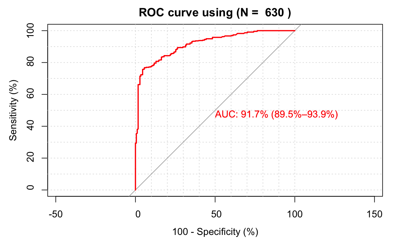
Figure 7.5: Application of the ROC methodology on the fishing-mode dataset.