7 Models of Count Data
Count-data models aim at explaining dependent variables \(y_i\) that take integer values. Typically, one may want to account for the number of doctor visits, of customers, of hospital stays, of borrowers’ defaults, of recreational trips, of accidents. Quite often, these data feature large proportion of zeros (see, e.g., Table 20.1 in Cameron and Trivedi (2005)), and/or are skewed to the right.
7.1 Poisson model
The most basic count-data model is the Poisson model. In this model, we have \(y \sim \mathcal{P}(\mu)\), i.e. \[ \mathbb{P}(y=k) = \frac{\mu^k e^{-\mu}}{k!}, \] implying \(\mathbb{E}(y) = \mathbb{V}ar(y) = \mu\).
the Poisson parameter, \(\mu\), is then assumed to depend on some observed variables, gathered in vector \(\mathbf{x}_i\) for entity \(i\). To ensure that \(\mu_i \ge 0\), it is common to take \(\mu_i = \exp(\boldsymbol\beta'\mathbf{x}_i)\), which gives: \[ y_i \sim \mathcal{P}(\exp[\boldsymbol\beta'\mathbf{x}_i]). \]
The Poisson regression is intrinsically heteroskedastic (since \(\mathbb{V}ar(y_i) = \mu_i = \exp(\boldsymbol\beta'\mathbf{x}_i)\)).
Under the assumption of independence across entities, the log-likelihood is given by: \[ \log \mathcal{L}(\boldsymbol\beta;\mathbf{y},\mathbf{X}) = \sum_{i=1}^n (y_i \boldsymbol\beta'\mathbf{x}_i - \exp[\boldsymbol\beta'\mathbf{x}_i] - \ln[y_i!]). \] The first-order condition to get the MLE is: \[\begin{equation} \sum_{i=1}^n (y_i - \exp[\boldsymbol\beta'\mathbf{x}_i])\mathbf{x}_i = \underbrace{\mathbf{0}}_{K \times 1}. \tag{7.1} \end{equation}\]
Eq. (7.1) is equivalent to what would define the Pseudo Maximum-Likelihood estimator of \(\boldsymbol\beta\) in the (misspecified) model \[ y_i \sim i.i.d.\,\mathcal{N}(\exp[\boldsymbol\beta'\mathbf{x}_i],\sigma^2). \] That is, Eq. (7.1) also characterizes the (true) ML estimator of \(\boldsymbol\beta\) in the previous model.
Since \(\mathbb{E}(y_i|\mathbf{x}_i) = \exp(\boldsymbol\beta'\mathbf{x}_i)\), we have: \[ y_i = \exp(\boldsymbol\beta'\mathbf{x}_i) + \varepsilon_i, \] with \(\mathbb{E}(\varepsilon_i|\mathbf{x}_i) = 0\). This notably implies that the (N)LS estimator of \(\boldsymbol\beta\) is consistent.
How to interpret regression coefficients (the components of \(\boldsymbol\beta\))? We have: \[ \frac{\partial \mathbb{E}(y_i|\mathbf{x}_i)}{\partial x_{i,j}} = \beta_j \exp(\boldsymbol\beta'\mathbf{x}_i), \] which depends on the considered individual.
The average estimated response is: \[ \widehat{\beta}_j \frac{1}{n}\sum_{i=1}^n \exp(\widehat{\boldsymbol\beta}'\mathbf{x}_i), \] which is equal to \(\widehat{\beta}_j \overline{y}\) if the model includes a constant (e.g., if \(x_{1,i}=1\) for all entities \(i\)).
The limitation of the standard Poisson model is that the distribution of \(y_i\) conditional on \(\mathbf{x}_i\) depends on a single parameter (\(\mu_i\)). Besides, there is often a tension between fitting the fraction of zeros, i.e. \(\mathbb{P}(y_i=0|\mathbf{x}_i)=\exp[-\exp(\boldsymbol\beta'\mathbf{x}_i)]\), and the distribution of \(y_i|\mathbf{x}_i,y_i>0\). The following models (negative binomial, or NB model, the Hurdle model, and the Zero-Inflated model) have been designed to address these points.
7.2 Negative binomial model
In the negative binomial model, we have: \[ y_i|\lambda_i \sim \mathcal{P}(\lambda_i), \] but \(\lambda_i\) is now random. Specifically, it takes the form: \[ \lambda_i = \nu_i \times \exp(\boldsymbol\beta'\mathbf{x}_i), \] where \(\nu_i \sim \,i.i.d.\,\Gamma(\underbrace{\delta}_{\mbox{shape}},\underbrace{1/\delta}_{\mbox{scale}})\). That is, the p.d.f. of \(\nu_i\) is: \[ g(\nu) = \frac{\nu^{\delta - 1}e^{-\nu\delta}\delta^\delta}{\Gamma(\delta)}, \] where \(\Gamma:\,z \mapsto \int_0^{+\infty}t^{z-1}e^{-t}dt\) (and \(\Gamma(k+1)=k!\)).
This notably implies that: \[ \mathbb{E}(\nu_i) = 1 \quad \mbox{and} \quad \mathbb{V}ar(\nu) = \frac{1}{\delta}. \]
Hence, the p.d.f. of \(y_i\) conditional on \(\mu\) and \(\delta\) (with \(\mu=\exp(\boldsymbol\beta'\mathbf{x}_i)\)) is obtained as a mixture of densities: \[ \mathbb{P}(y_i=k|\exp(\boldsymbol\beta'\mathbf{x}_i)=\mu;\delta)=\int_0^\infty \frac{e^{-\mu \nu}(\mu \nu)^k}{k!} \frac{\nu^{\delta - 1}e^{-\nu\delta}\delta^\delta}{\Gamma(\delta)} d \nu. \]
It can be shown that: \[ \mathbb{E}(y|\mathbf{x}) = \mu \quad \mbox{and}\quad \mathbb{V}ar(y|\mathbf{x}) = \mu\left(1+\alpha \mu\right), \] where \(\exp(\boldsymbol\beta'\mathbf{x}_i)=\mu\) and \(\alpha = 1/\delta\).
We have one additional degree of freedom w.r.t. the Poisson model (\(\alpha\)).
Note that \(\mathbb{V}ar(y|\mathbf{x}) > \mathbb{E}(y|\mathbf{x})\) (which is often called for by the data). Moreover, the conditional variance is quadratic in the mean: \[ \mathbb{V}ar(y|\mathbf{x}) = \mu+\alpha \mu^2. \] The previous expression is the basis of the so-called NB2 specification. If \(\delta\) is replaced with \(\mu/\gamma\), then we get the NB1 model: \[ \mathbb{V}ar(y|\mathbf{x}) = \mu(1+\gamma). \]
Example 7.1 (Number of doctor visits) The following example compares different specifications, namely a linear regression model, a Poisson model, and a NB model, to account for the number of doctor visits. The dataset (`randdata) is the one used in Chapter 20 of Cameron and Trivedi (2005) (available on that page).
library(AEC)
library(COUNT)
library(pscl) # for predprob function and hurdle model
par(plt=c(.15,.95,.1,.95))
plot(table(randdata$mdvis))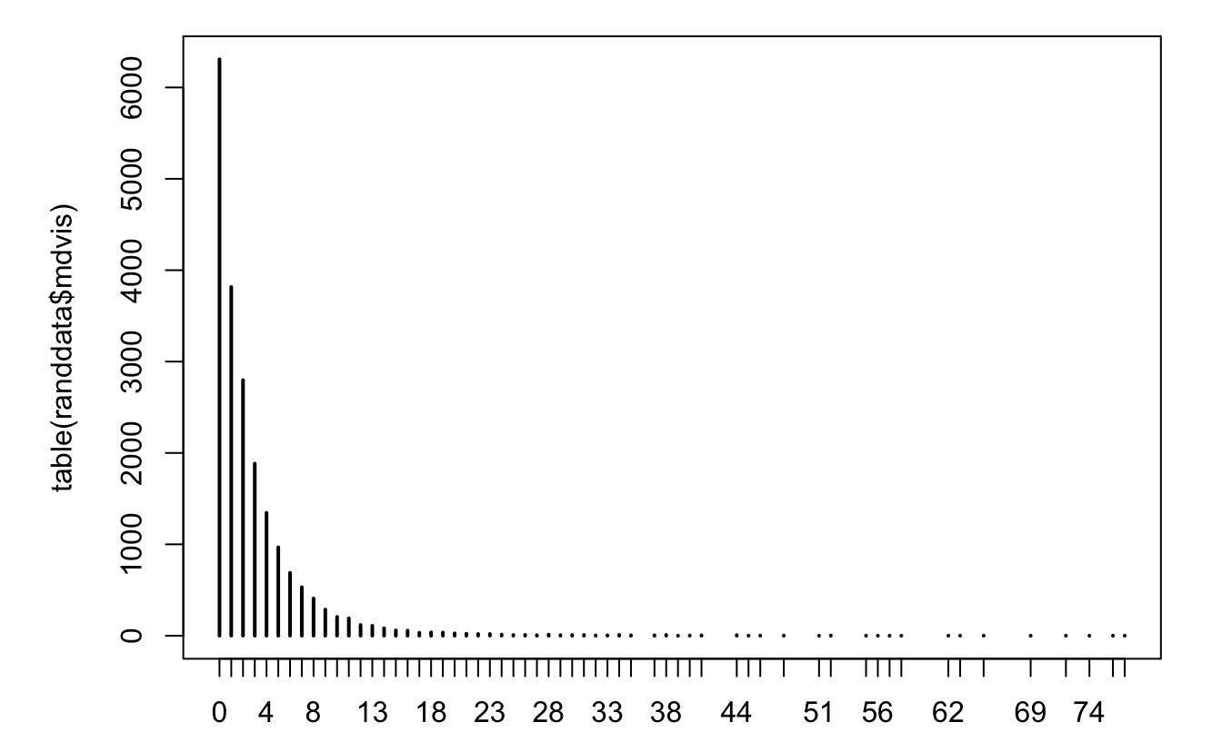
Figure 7.1: Distribution of the number of doctor visits.
## [1] 2.860426 20.289300As shown on the previous line, the variance of the number of visits is much larger than its expectation. This suggests that a Poisson model would be misspecified.
randdata$LC <- log(1 + randdata$coins)
model.OLS <- lm(mdvis ~ LC + idp + lpi + fmde + physlm + disea + hlthg +
                  hlthf + hlthp - 1,data=randdata)
model.poisson <- glm(mdvis ~ LC + idp + lpi + fmde + physlm + disea +
                       hlthg + hlthf + hlthp - 1,data=randdata,family = poisson)
model.neg.bin <- glm.nb(mdvis ~ LC + idp + lpi + fmde + physlm + disea +
                          hlthg + hlthf + hlthp - 1,data=randdata)
model.neg.bin.with.intercept <-
  glm.nb(mdvis ~ LC + idp + lpi + fmde + physlm + disea + hlthg +
           hlthf + hlthp,data=randdata)
stargazer::stargazer(model.OLS,model.poisson,model.neg.bin,
                     model.neg.bin.with.intercept,type="text",
                     no.space = TRUE,omit.stat = c("f","ser"))
##
## =========================================================================
## Dependent variable:
## -------------------------------------------------------
## mdvis
## OLS Poisson negative
## binomial
## (1) (2) (3) (4)
## -------------------------------------------------------------------------
## LC -0.155*** -0.051*** -0.057*** -0.058***
## (0.020) (0.003) (0.006) (0.006)
## idp -0.546*** -0.183*** -0.212*** -0.268***
## (0.075) (0.011) (0.023) (0.023)
## lpi 0.230*** 0.095*** 0.088*** 0.041***
## (0.012) (0.002) (0.004) (0.004)
## fmde -0.073*** -0.029*** -0.030*** -0.038***
## (0.012) (0.002) (0.004) (0.003)
## physlm 0.945*** 0.217*** 0.229*** 0.269***
## (0.104) (0.013) (0.031) (0.030)
## disea 0.177*** 0.050*** 0.062*** 0.038***
## (0.004) (0.0005) (0.001) (0.001)
## hlthg 0.270*** 0.126*** 0.068*** -0.044**
## (0.066) (0.009) (0.020) (0.020)
## hlthf 0.455*** 0.149*** 0.084** 0.017
## (0.123) (0.016) (0.037) (0.036)
## hlthp 1.537*** 0.197*** 0.185** 0.178**
## (0.263) (0.027) (0.076) (0.074)
## Constant 0.664***
## (0.025)
## -------------------------------------------------------------------------
## Observations 20,190 20,190 20,190 20,190
## R2 0.322
## Adjusted R2 0.322
## Log Likelihood -64,221.340 -43,745.860 -43,384.660
## theta 0.732*** (0.010) 0.773*** (0.011)
## Akaike Inf. Crit. 128,460.700 87,509.710 86,789.320
## =========================================================================
## Note: *p<0.1; **p<0.05; ***p<0.01In the previous table, The reported \(\theta\) is the inverse of \(\alpha\) appearing in \(\mathbb{V}ar(y|\mathbf{x}) = \mu+\alpha \mu^2\) (NB2 specification). That is, the model implies that \(\mathbb{V}ar(y|\mathbf{x}) = \mu+\mu^2/\theta\).
Models’ predictions can be obtained as follows:
# prediction of beta'x, equivalent to "model.poisson$fitted.values":
predict_poisson.beta.x <- predict(model.poisson)
# prediction of the number of events (exp(beta'x)):
predict_poisson <- predict(model.poisson,type="response")
predict_NB <- model.neg.bin$fitted.values
Let us now compute the model-implied probabilities, and let’s compare them with the frequencies observed in the data.
prop.table.data  <- prop.table(table(randdata$mdvis))
predprob.poisson <- predprob(model.poisson) # part of pscl package
predprob.nb      <- predprob(model.neg.bin)
print(rbind(prop.table.data[1:6],
            apply(predprob.poisson[,1:6],2,mean),
            apply(predprob.nb[,1:6],2,mean)))
## 0 1 2 3 4 5
## [1,] 0.3124319 0.1890540 0.1385339 0.09331352 0.06661714 0.04794453
## [2,] 0.1220592 0.2230328 0.2271621 0.17173478 0.10888940 0.06244353
## [3,] 0.3486824 0.1884640 0.1219340 0.08385899 0.05968603 0.04350209It appears that the NB model is better at capturing the relatively large number of zeros than the Poisson model. This will also be the case for the Hurdle and Zero-Inflation models:
7.3 Hurdle model
The main objective of this model, w.r.t. the Poisson model, is to generate more zeros in the data than predicted by the previous count models. The idea is to separate the modeling of the number of zeros and that of the number of non-zero counts. Specifically, the frequency of zeros is determined by \(f_1\), the (relative) frequencies of non-zero counts are determined by \(f_2\): \[ f(y) = \left\{ \begin{array}{lll} f_1(0) & \mbox{if $y=0$},\\ \dfrac{1-f_1(0)}{1-f_2(0)}f_2(y) & \mbox{if $y>0$}. \end{array} \right. \]
Note that we are back to the standard Poisson model if \(f_1 \equiv f_2\). This model is straightforwardly estimated by ML.
7.4 Zero-inflated model
The objective is the same as for the Hurdle model, the modeling is slightly different. It is based on a mixture of a binary process \(B\) (p.d.f. \(f_1\)) and a process \(Z\) (p.d.f. \(f_2\)). \(B\) and \(Z\) are independent. Formally: \[ y = B Z, \] implying: \[ f(y) = \left\{ \begin{array}{lll} f_1(0) + (1-f_1(0))f_2(0) & \mbox{if $y=0$},\\ (1-f_1(0))f_2(y) & \mbox{if $y>0$}. \end{array} \right. \] Typically, \(f_1\) corresponds to a logit model and \(f_2\) is Poisson or negative binomial density. This model is easily estimated by ML techniques.
Example 7.2 (Number of doctor visits) Let us come back to the data used in Example 7.1, and estimate Hurdle and a zero-inflation models:
library(stargazer)
model.hurdle <-
  hurdle(mdvis ~ LC + idp + lpi + fmde + physlm + disea + hlthg + hlthf +
           hlthp, data=randdata,
         dist = "poisson", zero.dist = "binomial", link = "logit")
model.zeroinfl <- zeroinfl(mdvis ~ LC + idp + lpi + fmde + physlm +
                             disea + hlthg + hlthf + hlthp, data=randdata,
                           dist = "poisson", link = "logit")
stargazer(model.hurdle,model.zeroinfl,zero.component=FALSE,
          no.space=TRUE,type="text")
##
## ===========================================
## Dependent variable:
## ----------------------------
## mdvis
## hurdle zero-inflated
## count data
## (1) (2)
## -------------------------------------------
## LC -0.015*** -0.015***
## (0.003) (0.003)
## idp -0.085*** -0.086***
## (0.011) (0.011)
## lpi 0.010*** 0.010***
## (0.002) (0.002)
## fmde -0.021*** -0.021***
## (0.002) (0.002)
## physlm 0.231*** 0.231***
## (0.012) (0.012)
## disea 0.022*** 0.022***
## (0.001) (0.001)
## hlthg 0.027*** 0.026***
## (0.010) (0.010)
## hlthf 0.147*** 0.146***
## (0.016) (0.016)
## hlthp 0.304*** 0.303***
## (0.026) (0.026)
## Constant 1.133*** 1.133***
## (0.012) (0.012)
## -------------------------------------------
## Observations 20,190 20,190
## Log Likelihood -54,772.100 -54,772.550
## ===========================================
## Note: *p<0.1; **p<0.05; ***p<0.01
stargazer(model.hurdle,model.zeroinfl,zero.component=TRUE,
          no.space=TRUE,type="text")
##
## ===========================================
## Dependent variable:
## ----------------------------
## mdvis
## hurdle zero-inflated
## count data
## (1) (2)
## -------------------------------------------
## LC -0.150*** 0.154***
## (0.010) (0.011)
## idp -0.631*** 0.637***
## (0.038) (0.040)
## lpi 0.102*** -0.105***
## (0.007) (0.007)
## fmde -0.062*** 0.060***
## (0.006) (0.006)
## physlm 0.239*** -0.203***
## (0.056) (0.058)
## disea 0.062*** -0.059***
## (0.003) (0.003)
## hlthg -0.142*** 0.158***
## (0.034) (0.036)
## hlthf -0.352*** 0.396***
## (0.062) (0.064)
## hlthp -0.181 0.233
## (0.149) (0.151)
## Constant 0.411*** -0.528***
## (0.044) (0.047)
## -------------------------------------------
## Observations 20,190 20,190
## Log Likelihood -54,772.100 -54,772.550
## ===========================================
## Note: *p<0.1; **p<0.05; ***p<0.01Let us test the importance of LC in the model using a Wald test:
# Test whether LC is important in the model:
model.hurdle.reduced <- update(model.hurdle,.~.-LC)
lmtest::waldtest(model.hurdle, model.hurdle.reduced)
## Wald test
##
## Model 1: mdvis ~ LC + idp + lpi + fmde + physlm + disea + hlthg + hlthf +
## hlthp
## Model 2: mdvis ~ idp + lpi + fmde + physlm + disea + hlthg + hlthf + hlthp
## Res.Df Df Chisq Pr(>Chisq)
## 1 20170
## 2 20172 -2 247.64 < 2.2e-16 ***
## ---
## Signif. codes: 0 '***' 0.001 '**' 0.01 '*' 0.05 '.' 0.1 ' ' 1Finally, we compare average model-implied probabilities with the frequencies observed in the data:
predprob.hurdle   <- predprob(model.hurdle)
predprob.zeroinfl <- predprob(model.zeroinfl)
print(rbind(prop.table.data[1:6],
  apply(predprob.poisson[,1:6],2,mean),
  apply(predprob.nb[,1:6],2,mean),
  apply(predprob.hurdle[,1:6],2,mean),
  apply(predprob.zeroinfl[,1:6],2,mean)))
## 0 1 2 3 4 5
## [1,] 0.3124319 0.18905399 0.1385339 0.09331352 0.06661714 0.04794453
## [2,] 0.1220592 0.22303277 0.2271621 0.17173478 0.10888940 0.06244353
## [3,] 0.3486824 0.18846395 0.1219340 0.08385899 0.05968603 0.04350209
## [4,] 0.3124319 0.06056959 0.1083120 0.13262624 0.12553899 0.09847017
## [5,] 0.3124687 0.06053019 0.1082797 0.13262552 0.12556525 0.09850216