5 Multiple Choice Models

We will now consider cases where the number of possible outcomes (or alternatives) is larger than two. Let us denote by \(J\) this number. We have \(y_j \in \{1,\dots,J\}\). This situation arise for instance when the outcome variable reflects:

• Opinions: strongly opposed / opposed / neutral / support (ranked choices),
• Occupational field: lawyer / farmer / engineer / doctor / …,
• Alternative shopping areas,
• Transportation types.

In a few cases, the values associated with the choices will themselves be meaningful, for example, number of accidents per day: \(y = 0, 1,2, \dots\) (count data). In most cases, the values are meaningless.

We assume the existence of covariates, gathered in vector \(\mathbf{x}_i\) (\(K \times 1\)), that are suspected to influence for the probabilities of obtaining the different outcomes (\(y_i=j\), \(j \in \{1,\dots,J\}\)).

In what follows, we will assume that the \(y_i\)’s are assumed to be independently distributed, with: \[\begin{equation} y_i = \left\{ \begin{array}{cl} 1 & \mbox{ with probability } g_1(\mathbf{x}_i;\boldsymbol\theta)\\ \vdots \\ J & \mbox{ with probability } g_J(\mathbf{x}_i;\boldsymbol\theta). \end{array} \right.\tag{5.1} \end{equation}\]

(Of course, for all entities (\(i\)), we must have \(\sum_{j=1}^J g_j(\mathbf{x}_i;\boldsymbol\theta)=1\).) Our objective is to estimate the vector of population parameters \(\boldsymbol\theta\) given functional forms for the \(g_j\)’s.

5.1 Ordered case

Sometimes, there exists a natural order for the different alternatives. This is typically the case where respondents have to choose a level of agreement to a statement, e.g.: (1) Strongly disagree; (2) Disagree; (3) Neither agree nor disagree; (4) Agree; (5) Strongly agree. Another standard case is that of ratings (from A to F, say).

The ordered probit model consists in extending the binary case, considering the latent-variable view of the latter (see Section 4.1). Formally, the model is as follows: \[\begin{equation} \mathbb{P}(y_i = j | \mathbf{x}_i) = \mathbb{P}(\alpha_{j-1} <y^*_i < \alpha_{j} |\mathbf{x}_i), \tag{5.2} \end{equation}\] where \[ y_{i}^* = \boldsymbol\theta'\mathbf{x}_i + \varepsilon_i, \] with \(\varepsilon_i \sim \,i.i.d.\,\mathcal{N}(0,1)\). The \(\alpha_j\)’s, \(j \in \{1,\dots,J-1\}\), are (new) parameters that have to be estimated, on top of \(\boldsymbol\theta\). Naturally, we have \(\alpha_1<\alpha_2<\dots<\alpha_{J-1}\). Moreover \(\alpha_0\) is \(- \infty\) and \(\alpha_J\) is \(+ \infty\), so that Eq. (5.2) is valid for any \(j \in \{1,\dots,J\}\) (including \(1\) and \(J\)).

We have: \[\begin{eqnarray*} g_j(\mathbf{x}_i;\boldsymbol\theta,\boldsymbol\alpha) = \mathbb{P}(y_i = j | \mathbf{x}_i) &=& \mathbb{P}(\alpha_{j-1} <y^*_i < \alpha_{j} |\mathbf{x}_i) \\ &=& \mathbb{P}(\alpha_{j-1} - \boldsymbol\theta'\mathbf{x}_i <\varepsilon_i < \alpha_{j} - \boldsymbol\theta'\mathbf{x}_i) \\ &=& \Phi(\alpha_{j} - \boldsymbol\theta'\mathbf{x}_i) - \Phi(\alpha_{j-1} - \boldsymbol\theta'\mathbf{x}_i), \end{eqnarray*}\] where \(\Phi\) is the c.d.f. of \(\mathcal{N}(0,1)\).

If, for all \(i\), one of the components of \(\mathbf{x}_i\) is equal to 1 (which is what is done in linear regression to introduce an intercept in the specification), then one of the \(\alpha_j\) (\(j\in\{1,\dots,J-1\}\)) is not identified. One can then arbitrarily set \(\alpha_1=0\). This is what is done in the binary logit/probit cases.

This model can be estimated by maximizing the likelihood function (see Section 3.2). This function is given by: \[\begin{equation} \log \mathcal{L}(\boldsymbol\theta,\boldsymbol\alpha;\mathbf{y},\mathbf{X}) = \sum_{i=1}^n \sum_{j=1}^J \mathbb{I}_{\{y_i=j\}} \log \left(g_j(\mathbf{x}_i;\boldsymbol\theta,\boldsymbol\alpha)\right). \tag{5.3} \end{equation}\]

Let us stress that we have two types of parameters to estimate: those included in vector \(\boldsymbol\theta\), and the \(\alpha_j\)’s, gathered in vector \(\boldsymbol\alpha\).

The estimated values of the \(\theta_j\)’s are slightly more complicated to interpret (at least in term of sign) than in the binary case. Indeed, we have: \[ \mathbb{P}(y_i \le j | \mathbf{x}_i) = \Phi(\alpha_{j} - \boldsymbol\theta'\mathbf{x}_i) \Rightarrow \frac{\partial \mathbb{P}(y_i \le j | \mathbf{x}_i)}{\partial\mathbf{x}_i} =- \underbrace{\Phi'(\alpha_{j} - \boldsymbol\theta'\mathbf{x}_i)}_{>0}\boldsymbol\theta. \] Hence the sign of \(\theta_k\) indicates whether \(\mathbb{P}(y_i \le j | \mathbf{x}_i)\) increases or decreases w.r.t. \(x_{i,k}\) (the \(k^{th}\) component of \(\mathbf{x}_i\)). By contrast: \[ \frac{\partial \mathbb{P}(y_i = j | \mathbf{x}_i)}{\partial\mathbf{x}_i} = \underbrace{\left(-\Phi'(\alpha_{j} + \boldsymbol\theta'\mathbf{x}_i)+\Phi'(\alpha_{j-1} + \boldsymbol\theta'\mathbf{x}_i)\right)}_{A}\boldsymbol\theta. \] Therefore the signs of the components of \(\boldsymbol\theta\) are not necessarily those of the marginal effects. (For the sign of \(A\) is a priori unknown.)

Example 5.1 (Predicting credit ratings (Lending-club dataset)) Let us use credit dataset again (see Example 4.3), and let use try and model the ratings attributed by the lending-club:

library(AEC)
library(MASS)
credit$emp_length_low5y   <- credit$emp_length %in%
  c("< 1 year","1 year","2 years","3 years","4 years")
credit$emp_length_high10y <- credit$emp_length=="10+ years"
credit$annual_inc <- credit$annual_inc/1000
credit$loan_amnt  <- credit$loan_amnt/1000
credit$income2loan <- credit$annual_inc/credit$loan_amnt
training <- credit[1:20000,] # sample is reduced
training <- subset(training,grade!=c("E","F","G"))
training <- droplevels(training)
training$grade.ordered <- factor(training$grade,ordered=TRUE,
                                 levels = c("D","C","B","A"))
model1 <- polr(grade.ordered ~ log(loan_amnt) + log(income2loan) + delinq_2yrs,
               data=training, Hess=TRUE, method="probit")
model2 <- polr(grade.ordered ~ log(loan_amnt) + log(income2loan) + delinq_2yrs +
                 emp_length_low5y + emp_length_high10y,
               data=training, Hess=TRUE, method="probit")
stargazer::stargazer(model1,model2,ord.intercepts = TRUE,type="text",
                     no.space = TRUE)

## 
## ===============================================
##                        Dependent variable:     
##                    ----------------------------
##                           grade.ordered        
##                         (1)            (2)     
## -----------------------------------------------
## log(loan_amnt)         -0.014        -0.040*   
##                       (0.022)        (0.022)   
## log(income2loan)      0.115***      0.092***   
##                       (0.022)        (0.022)   
## delinq_2yrs          -0.399***      -0.404***  
##                       (0.025)        (0.025)   
## emp_length_low5y                    -0.096***  
##                                      (0.027)   
## emp_length_high10y                   0.088**   
##                                      (0.035)   
## D| C                 -0.937***      -1.073***  
##                       (0.082)        (0.086)   
## C| B                  -0.160**      -0.295***  
##                       (0.082)        (0.085)   
## B| A                  0.696***      0.564***   
##                       (0.082)        (0.086)   
## -----------------------------------------------
## Observations           8,695          8,695    
## ===============================================
## Note:               *p<0.1; **p<0.05; ***p<0.01

Predicted ratings (and probabilties of being given a given rating) can be computed as follows:

pred.grade <- predict(model1,newdata = training)
# pred.grade = predicted grade, defined as the most likely according model
pred.proba <- predict(model1,newdata = training, type="probs")

5.2 General multinomial logit model

This section introduces the general multinomial logit model, which is the natural extension of the binary logit model (see Table 4.1). Its general formulation is as follows: \[\begin{equation} g_j(\mathbf{x}_i;\boldsymbol\theta) = \frac{\exp(\theta_j'\mathbf{x}_i)}{\sum_{k=1}^J \exp(\theta_k'\mathbf{x}_i)}.\tag{5.4} \end{equation}\]

Note that, by construction, \(g_j(\mathbf{x}_i;\boldsymbol\theta) \in [0,1]\) and \(\sum_{j}g_j(\mathbf{x}_i;\boldsymbol\theta)=1\).

The components of \(\mathbf{x}_i\) (regressors, or covariates) may be alternative-specific or alternative invariant (see also Section 4.2). We may, e.g., organize \(\mathbf{x}_i\) as follows: \[\begin{equation} \mathbf{x}_i = [\mathbf{u}_{i,1}',\dots,\mathbf{u}_{i,J}',\mathbf{v}_{i}']',\tag{5.5} \end{equation}\] where the notations are as in Section 4.2, that is:

• \(\mathbf{u}_{i,j}\) (\(j \in \{1,\dots,J\}\)): vector of variables associated with agent \(i\) and alternative \(j\) (alternative-specific regressors). Examples: Travel time per type of transportation (transportation choice), wage per type of work, cost per type of car.
• \(\mathbf{v}_{i}\): vector of variables associated with agent \(i\) but alternative-invariant. Examples: age or gender of agent \(i\),

When \(\mathbf{x}_i\) is as in Eq. (5.5), with obvious notations, \(\theta_j\) is of the form: \[\begin{equation} \theta_j = [{\theta^{(u)}_{1,j}}',\dots,{\theta^{(u)}_{J,j}}',{\theta_j^{(v)}}']',\tag{5.6} \end{equation}\] and \(\boldsymbol\theta=[\theta_1',\dots,\theta_J']'\).

The literature has considered different specific cases of the general multinomial logit model:¹⁴

• Conditional logit (CL) with alternative-varying regressors: \[\begin{equation} \theta_j = [\mathbf{0}',\dots,\mathbf{0}',\underbrace{\boldsymbol\beta'}_{\mbox{j$^{th}$ position}},\mathbf{0}',\dots]',\tag{5.7} \end{equation}\] i.e., we have \(\boldsymbol\beta=\theta^{(u)}_{1,1}=\dots=\theta^{(u)}_{J,J}\) and \(\theta^{(u)}_{i,j}=\mathbf{0}\) for \(i \ne j\).
• Multinomial logit (MNL) with alternative-invariant regressors: \[\begin{equation} \theta_j = \left[\mathbf{0}',\dots,\mathbf{0}',{\theta_j^{(v)}}'\right]'.\tag{5.8} \end{equation}\]
• Mixed logit: \[\begin{equation} \theta_j = \left[\mathbf{0}',\dots,\mathbf{0}',\boldsymbol\beta',\mathbf{0}',\dots,\mathbf{0}',{\theta_j^{(v)}}'\right]'.\tag{5.7} \end{equation}\]

Example 5.2 (CL and MNL with the fishing-mode dataset) The following lines replicate Table 15.2 in Cameron and Trivedi (2005) (see also Examples 4.2 and 4.4):

# Specify data organization:
library(mlogit)
library(stargazer)
data("Fishing",package="mlogit")
Fish <- mlogit.data(Fishing,
                    varying = c(2:9),
                    choice = "mode",
                    shape = "wide")
MNL1 <- mlogit(mode ~ price + catch, data = Fish)
MNL2 <- mlogit(mode ~ price + catch - 1, data = Fish)
MNL3 <- mlogit(mode ~ 0 | income, data = Fish)
MNL4 <- mlogit(mode ~ price + catch | income, data = Fish)
stargazer(MNL1,MNL2,MNL3,MNL4,type="text",no.space = TRUE,
          omit.stat = c("lr"))

## 
## ===============================================================
##                                 Dependent variable:            
##                     -------------------------------------------
##                                        mode                    
##                        (1)        (2)        (3)        (4)    
## ---------------------------------------------------------------
## (Intercept):boat     0.871***              0.739***   0.527**  
##                      (0.114)               (0.197)    (0.223)  
## (Intercept):charter  1.499***              1.341***   1.694*** 
##                      (0.133)               (0.195)    (0.224)  
## (Intercept):pier     0.307***              0.814***   0.778*** 
##                      (0.115)               (0.229)    (0.220)  
## price               -0.025***  -0.020***             -0.025*** 
##                      (0.002)    (0.001)               (0.002)  
## catch                0.377***   0.953***              0.358*** 
##                      (0.110)    (0.089)               (0.110)  
## income:boat                                0.0001**   0.0001*  
##                                           (0.00004)   (0.0001) 
## income:charter                             -0.00003   -0.00003 
##                                           (0.00004)   (0.0001) 
## income:pier                               -0.0001*** -0.0001** 
##                                            (0.0001)   (0.0001) 
## ---------------------------------------------------------------
## Observations          1,182      1,182      1,182      1,182   
## R2                    0.178      0.014      0.189              
## Log Likelihood      -1,230.784 -1,311.980 -1,477.151 -1,215.138
## ===============================================================
## Note:                               *p<0.1; **p<0.05; ***p<0.01

ML estimation

General multinomial logit models can be estimated by Maximum Likelihood techniques (see Section 3.2). Consider the general model described in Eq. (5.1). It can be noted that: \[ f(y_i|\mathbf{x}_i;\boldsymbol\theta) = \prod_{j=1}^J g_j(\mathbf{x}_i;\boldsymbol\theta)^{\mathbb{I}_{\{y_i=j\}}}, \] which leads to \[ \log f(y_i|\mathbf{x}_i;\boldsymbol\theta) = \sum_{j=1}^J \mathbb{I}_{\{y_i=j\}} \log \left(g_j(\mathbf{x}_i;\boldsymbol\theta)\right). \] The log-likelihood function is therefore given by: \[\begin{equation} \log \mathcal{L}(\boldsymbol\theta;\mathbf{y},\mathbf{X}) = \sum_{i=1}^n \sum_{j=1}^J \mathbb{I}_{\{y_i=j\}} \log \left(g_j(\mathbf{x}_i;\boldsymbol\theta)\right).\tag{5.3} \end{equation}\] Numerical methods have to be employed in order to find the maximum-likelihood estimate of \(\boldsymbol\theta\). (Standard packages contain fast algorithms.)

Marginal Effects

Let us consider the computation of marginal effects in the general multinomial logit model (Eq. (5.4)). Using the notation \(p_{i,j} \equiv \mathbb{P}(y_i=j|\mathbf{x}_i;\boldsymbol\theta)\), we have: \[\begin{eqnarray*} \frac{\partial p_{i,j}}{\partial x_{i,s}} &=& \frac{\theta_{j,s}\exp(\theta_j'\mathbf{x}_i)\sum_{k=1}^J \exp(\theta_k'\mathbf{x}_i)}{(\sum_{k=1}^J \exp(\theta_k'\mathbf{x}_i))^2} \\ && - \frac{\exp(\theta_j'\mathbf{x}_i)\sum_{k=1}^J \theta_{k,s} \exp(\theta_k'\mathbf{x}_i)}{(\sum_{k=1}^J \exp(\theta_k'\mathbf{x}_i))^2}\\ &=& \theta_{j,s} p_{i,j} - \sum_{k=1}^J \theta_{k,s} p_{i,j}p_{i,k}\\ &=& p_{i,j} \times \Big(\theta_{j,s} - \underbrace{\sum_{k=1}^J \theta_{k,s} p_{i,k}}_{=\overline{\boldsymbol{\theta}}^{(i)}_{s}}\Big), \end{eqnarray*}\] where \(\overline{\boldsymbol\theta}^{(i)}_{s}\) does not depend on \(j\). Note that the sign of the marginal effect is not necessarily that of \(\theta_{j,s}\).

Random Utility models

The general multinomial logit model may arise as the natural specification arising in structural contexts where agents compare (random) utilities associated with \(J\) potential outcomes (see Section 4.1 for the binary situation).

Let’s drop the \(i\) subscript for simplicity and assume that the utility derived form choosing \(j\) is given by \(U_j = V_j + \varepsilon_j\), where \(V_j\) is deterministic (may depend on observed covariates) and \(\varepsilon_j\) is stochastic. We have (with obvious notations): \[\begin{eqnarray*} \mathbb{P}(y=j) &=& \mathbb{P}(U_j>U_k,\,\forall k \ne j)\\ \mathbb{P}(y=j) &=& \mathbb{P}(U_k-U_j<0,\,\forall k \ne j)\\ \mathbb{P}(y=j) &=& \mathbb{P}(\underbrace{\varepsilon_k-\varepsilon_j}_{=:\tilde\varepsilon_{k,j}}<\underbrace{V_j - V_k}_{=:-\tilde{V}_{k,j}},\,\forall k \ne j). \end{eqnarray*}\]

The last expression is an \((J-1)\)-variate integral. While it has, in general, no analytical solution, Prop. 5.1 shows that it is the case when employing Gumbel distributions (see Def. 5.1).

Definition 5.1 (Gumbel distribution) The c.d.f. of the Gumbel distribution (\(\mathcal{W}\)) is: \[ F(u) = \exp(-\exp(-u)), \qquad f(u)=\exp(-u-\exp(u)). \]

Remark: if \(X\sim\mathcal{W}\), then \(\mathbb{E}(X)=0.577\) (Euler constant)¹⁵ and \(\mathbb{V}ar(X)=\pi^2/6\).

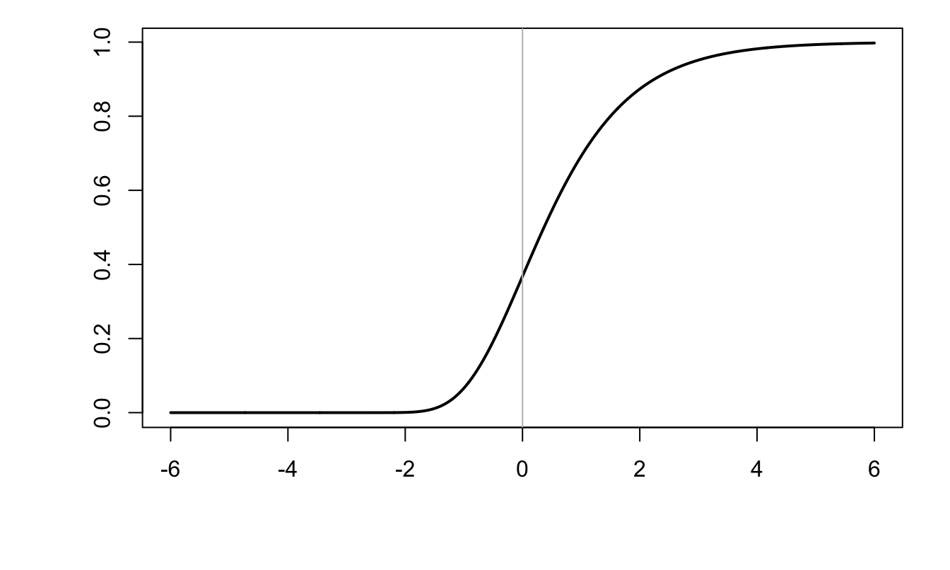
Figure 5.1: C.d.f. of the Gumbel distribution (\(F(x)=\exp(-\exp(-x))\)).

Proposition 5.1 (Weibull) In the context of the utility model described above, if \(\varepsilon_j \sim \,i.i.d.\,\mathcal{W}\), then \[ \mathbb{P}(y=j) = \frac{\exp(V_j)}{\sum_{k=1}^J \exp(V_k)}. \]

Proof. We have: \[\begin{eqnarray*} \mathbb{P}(y=j) &=& \mathbb{P}(\forall\,k \ne j,\,U_k < U_j) = \mathbb{P}(\forall\,k \ne j,\,\varepsilon_k < V_j - V_k + \varepsilon_j) \\ &=& \int \prod_{k \ne j} F(V_j - V_k + \varepsilon) f(\varepsilon)d\varepsilon. \end{eqnarray*}\] After computation, it comes that \[ \prod_{k \ne j} F(V_j - V_k + \varepsilon) f(\varepsilon) = \exp\left[-\varepsilon-\exp(-\varepsilon+\lambda_j)\right], \] where \(\lambda_j = \log\left(1 + \frac{\sum_{k \ne j} \exp(V_k)}{\exp(V_j)}\right)\). We then have: \[\begin{eqnarray*} \mathbb{P}(y=j) &=& \int \exp\left[-\varepsilon-\exp(-\varepsilon+\lambda_j)\right] d\varepsilon\\ &=& \int \exp\left[-t - \lambda_j-\exp(-t)\right] d\varepsilon = \exp(- \lambda_j), \end{eqnarray*}\] which leads to the result.

Some remarks on identification (see Def. 3.5) are in order.

1. We have: \[\begin{eqnarray*} \mathbb{P}(y=j) &=& \frac{\exp(V_j)}{\sum_{k=1}^J \exp(V_k)}= \frac{\exp(V^*_j)}{1 + \sum_{k=2}^J \exp(V^*_k)}, \end{eqnarray*}\] where \(V^*_j = V_j - V_1\). We can therefore always assume that \(V_{1}=0\). In the case where \(V_{i,j} = \theta_j'\mathbf{x}_i = \boldsymbol\beta'\mathbf{u}_{i,j}+{\theta_j^{(v)}}'\mathbf{v}_i\) (see Eqs. (5.5) and (5.7)), we can for instance assume that: \[\begin{eqnarray*} &(A)& \mathbf{u}_{i,1}=0,\\ &(B)& \theta_1^{(v)} = 0. \end{eqnarray*}\] If (A) does not hold, we can replace \(\mathbf{u}_{i,j}\) with \(\mathbf{u}_{i,j}-\mathbf{u}_{i,1}\).
2. If \(J=2\) and \(j \in \{0,1\}\) (shift by one unit), we have \(\mathbb{P}(y=1|\mathbf{x})=\dfrac{\exp(\boldsymbol\theta'\mathbf{x})}{1+\exp(\boldsymbol\theta'\mathbf{x})}\), this is the logit model (Table 4.1).

Limitations of logit models

In a Logit model, we have: \[\begin{equation} \mathbb{P}(y=j|y \in \{k,j\}) = \frac{\exp(\theta_j'\mathbf{x})}{\exp(\theta_j'\mathbf{x}) + \exp(\theta_k'\mathbf{x})}.\tag{5.9} \end{equation}\] This conditional probability does not depend on other alternatives (i.e., it does not depend on \(\theta_m\), \(m \ne j,k\)). In particular, if \(\mathbf{x} = [\mathbf{u}_1',\dots,\mathbf{u}_J',\mathbf{v}']'\), then changes in \(\mathbf{u}_m\) (\(m \ne j,\,k\)) have no impact on the object shown in Eq. (5.9).

That is, a Multinomial Logit can be seen as a series of pairwise comparisons that are unaffected by the characteristics of alternatives. Such a model is said to satisfy the independence from irrelevant alternatives (IIA) property. That is, in these models, for any individual, the ratio of probabilities of choosing two alternatives is independent of the availability or attributes of any other alternatives. While this may not sound alarming, there are situations where you would like it not to be the case, this is for instance the case when you want to extrapolate the results of your estimated model to a situation where there is a novel outcome that is highly susbstitutable to one of the previous ones. This can be illustrated with the famous “red-blue bus” example:

Example 5.3 (Red-blue bus and IIA) Assume one has a logit model capturing the decision to travel using either a car (\(y=1\)) or a (red) bus (\(y=2\)). Assume you want to augment this model to allow for a third choice (\(y=3\)): travel with a blue bus. If a blue bus (\(y=3\)) is exactly as a red bus, except for the color, then one would expect to have: \[ \mathbb{P}(y=3|y \in \{2,3\}) = 0.5, \] i.e. \(\theta_2 = \theta_3\).

Assume we had \(V_1=V_2\). We expect to have \(V_2=V_3\) (hence \(p_2=p_3\)). A multinomial logit model would then imply \(p_1=p_2=p_3=0.33\). It would however seem more reasonable to have \(p_1 = p_2 + p_3 = 0.5\) and \(p_2=p_3=0.25\).

5.3 Nested logits

Nested Logits are natural extensions of logit models when choices feature a nesting structure. This approach is relevant when it makes sense to group some choices into the same nest, also called limbs. Intuitively, this framework is consistent with the idea according to which, for each agent, there exist unobserved nest-specific variables.

The setup is as follows: we consider \(J\) limbs. For each limb \(j\), we have \(K_j\) branches. Let us denotes by \(y_1\) the limb choice (i.e., \(y_1 \in \{1,\dots,J\}\)) and by \(y_2\) the branch choice (with \(y_2 \in \{1,\dots,K_j\}\)). The utility associated with the pair of choices \((j,k)\) is given by \[ U_{j,k} = V_{j,k} + \varepsilon_{j,k}. \] We have: \[ \mathbb{P}[(y_1,y_2) = (j,k)|\mathbf{x}] = \mathbb{P}(U_{j,k}>U_{l,m},\,(l,m) \ne (j,k)|\mathbf{x}). \]

One usually make the following two assumptions:

1. The deterministic part of the utility is given by \(V_{j,k} = \mathbf{u}_j'\boldsymbol\alpha + \mathbf{v}_{j,k}'\boldsymbol\beta_j\), where \(\boldsymbol\alpha\) is common to all nests and the \(\boldsymbol\beta_j\)’s are nest-specific.

2. The disturbances \(\boldsymbol\varepsilon\) follow the Generalized Extreme Value (GEV) distribution (see Def. 8.15).

The following figure displays simulations of pairs \((\varepsilon_1,\varepsilon_2)\) drawn from GEV distributions for different values of \(\rho\). The simulation approach is based on Bhat. The code used to produce this chart is provided in Appendix 8.5.1.

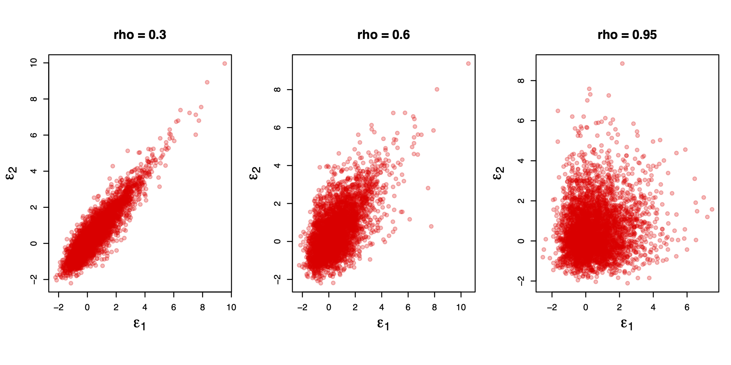
Figure 5.2: GEV simulations.

Under (i) and (ii), we have: \[\begin{eqnarray} \mathbb{P}[(y_1,y_2) = (j,k)|\mathbf{x}] &=& \underbrace{\frac{\exp(\mathbf{u}_j'\boldsymbol\alpha + \rho_j I_j)}{\sum_{m=1}^J \exp(\mathbf{u}_m'\boldsymbol\alpha + \rho_m I_m)}}_{= \mathbb{P}[y_1 = j|\mathbf{x}]} \times \nonumber\\ && \underbrace{\frac{\exp(\mathbf{v}_{j,k}'\boldsymbol\beta_j/\rho_j)}{\sum_{l=1}^{K_j} \exp(\mathbf{v}_{j,l}'\boldsymbol\beta_j/\rho_j)}}_{= \mathbb{P}[y_2 = k|y_1=j,\mathbf{x}]}, \tag{5.10} \end{eqnarray}\] where \(I_j\)’s are called inclusive values (or log sums), given by: \[ I_j = \log \left( \sum_{l=1}^{K_j} \exp(\mathbf{v}_{j,l}'\boldsymbol\beta_j/\rho_j)\right). \]

Some remarks are in order:

1. It can be shown that \(\rho_j = \sqrt{1 - \mathbb{C}or(\varepsilon_{j,k},\varepsilon_{j,l})}\), for \(k \ne l\).
2. \(\rho_j=1\) implies that \(\varepsilon_{j,k}\) and \(\varepsilon_{j,l}\) are uncorrelated (we are then back to the multinomial logit case).
3. When \(J=1\): \[ F([\varepsilon_1,\dots,\varepsilon_K]',\rho) = \exp\left(-\left(\sum_{k=1}^{K} \exp(-\varepsilon_k/\rho)\right)^{\rho}\right). \]
4. We have: \[\begin{eqnarray*} I_j = \mathbb{E}(\max_k(U_{j,k})) &=& \mathbb{E}(\max_k(V_{j,k} + \varepsilon_{j,k})), \end{eqnarray*}\] The inclusive values can therefore be seen as measures of the relative attractiveness of a nest.

This approach allows for some level of correlation across the \(\varepsilon_{j,k}\) (for a given \(j\)). This can be interpreted as the existence of an (unobserved) common error component for the alternatives of a same nest. This component contributes to making the alternatives of a given nest more similar. In other words, this approach can accommodate a higher sensitivity (cross-elasticity) between the alternatives of a given nest.

Note that if the common component is reduced to zero (i.e. \(\rho_i=1\)), the model boils down to the multinomial logit model with no covariance of error terms among the alternatives.

Contrary to the general multinomial model, nested logits can solve the Red-Blue problem described in Section 5.2 (see Example 5.3). Assume you have estimated a model specifying \(U_{1} = V_{1} + \varepsilon_{1}\) (car choice) and \(U_{2} = V_{2} + \varepsilon_{2}\) (red bus choice). You can then assume that the blue-bus utility is of the form \(U_{3} = V_{2} + \varepsilon_{3}\) where \(\varepsilon_{3}\) is perfectly correlated to \(\varepsilon_{2}\). This is done by redefining the set of choices as follows: \[\begin{eqnarray*} j=1 &\Leftrightarrow& (j'=1,k=1) \\ j=2 &\Leftrightarrow& (j'=2,k=1) \\ j=3 &\Leftrightarrow& (j'=2,k=2), \end{eqnarray*}\] and by setting \(\rho_2 \rightarrow 0\).

IIA holds within a nest, but not when considering alternatives in different nests. Indeed, using Eq. (5.10): \[ \frac{\mathbb{P}[y_1=j,y_2=k_A|\mathbf{x}] }{\mathbb{P}[y_1=j,y_2=k_B|\mathbf{x}]} = \frac{\exp(\mathbf{v}_{j,k_A}'\boldsymbol\beta_j/\rho_j)}{\exp(\mathbf{v}_{j,k_B}'\boldsymbol\beta_j/\rho_j)}, \] i.e. we have IIA in nest \(j\).

By contrast: \[\begin{eqnarray*} \frac{\mathbb{P}[y_1=j_A,y_2=k_A|\mathbf{x}] }{\mathbb{P}[y_1=j_B,y_2=k_B|\mathbf{x}]} &=& \frac{\exp(\mathbf{u}_{j_A}'\boldsymbol\alpha + \rho_{j_A} I_{j_A})\exp(\mathbf{v}_{{j_A},{k_A}}'\boldsymbol\beta_{j_A}/\rho_{j_A})}{\exp(\mathbf{u}_{j_B}'\boldsymbol\alpha + \rho_{j_B} I_{j_B})\exp(\mathbf{v}_{{j_B},{k_B}}'\boldsymbol\beta_{j_B}/\rho_{j_B})}\times\\ && \frac{\sum_{l=1}^{K_{j_B}} \exp(\mathbf{v}_{{j_B},l}'\boldsymbol\beta_{j_B}/\rho_{j_B})}{\sum_{l=1}^{K_{j_A}} \exp(\mathbf{v}_{{j_A},l}'\boldsymbol\beta_{J_A}/\rho_{j_A})}, \end{eqnarray*}\] which depends on the expected utilities of all alternatives in nest \(j_A\) and \(j_B\). So the IIA does not hold.

Example 5.4 (Travel-mode dataset) Let us illustrate nested logits on the travel-mode dataset used, e.g., by Hensher and Greene (2002) (see also Heiss (2002)).

library(mlogit)
library(stargazer)
data("TravelMode", package = "AER")
Prepared.TravelMode <- mlogit.data(TravelMode,chid.var = "individual",
                                   alt.var = "mode",choice = "choice",
                                   shape = "long")
# Fit a multinomial model:
hl <- mlogit(choice ~ wait + travel + vcost, Prepared.TravelMode,
             method = "bfgs", heterosc = TRUE, tol = 10)
## Fit a nested logit model:
TravelMode$avincome <- with(TravelMode, income * (mode == "air"))
TravelMode$time <- with(TravelMode, travel + wait)/60
TravelMode$timeair <- with(TravelMode, time * I(mode == "air"))
TravelMode$income <- with(TravelMode, income / 10)
# Hensher and Greene (2002), table 1 p.8-9 model 5
TravelMode$incomeother <- with(TravelMode,
                               ifelse(mode %in% c('air', 'car'), income, 0))
nl1 <- mlogit(choice ~ gcost + wait + incomeother, TravelMode,
              shape='long', # Indicates how the dataset is organized
              alt.var='mode', # variable that defines the alternative choices.
              nests=list(public=c('train', 'bus'),
                         car='car',air='air'), # defines the "limbs".
              un.nest.el = TRUE)
nl2 <- mlogit(choice ~ gcost + wait + time, TravelMode,
              shape='long', # Inidcates how the dataset is organized
              alt.var='mode', # variable that defines the alternative choices.
              nests=list(public=c('train', 'bus'),
                         car='car',air='air'), # defines the "limbs".
              un.nest.el = TRUE)
stargazer(nl1,nl2,type="text",no.space = TRUE)

## 
## ==============================================
##                       Dependent variable:     
##                   ----------------------------
##                              choice           
##                        (1)            (2)     
## ----------------------------------------------
## (Intercept):train     -0.211        -0.284    
##                      (0.562)        (0.551)   
## (Intercept):bus       -0.824        -0.712    
##                      (0.708)        (0.690)   
## (Intercept):car     -5.237***      -3.845***  
##                      (0.785)        (0.844)   
## gcost               -0.013***       -0.004    
##                      (0.004)        (0.006)   
## wait                -0.088***      -0.089***  
##                      (0.011)        (0.011)   
## incomeother          0.430***                 
##                      (0.113)                  
## time                               -0.202***  
##                                     (0.060)   
## iv                   0.835***      0.877***   
##                      (0.192)        (0.198)   
## ----------------------------------------------
## Observations           210            210     
## R2                    0.328          0.313    
## Log Likelihood       -190.779      -194.841   
## LR Test (df = 7)    185.959***    177.836***  
## ==============================================
## Note:              *p<0.1; **p<0.05; ***p<0.01