6 Tobit and sample-selection models
6.1 Tobit models
In some situations, the dependent variable is incompletely observed, which may result in a non-representative sample. Typically, in some cases, observations of the dependent variable can have a lower and/or an upper limit, while the “true”, underlying, dependent variable has not. In this case, OLS regression may lead to inconsistent parameter estimates.
Tobit models have been designed to address some of these situations. This approach has been named after James Tobin, who developed this model in the late 50s (see Tobin (1956)).
Figure 6.1 illustrates the situation. The dots (white and black) represent the “true” observations. Now, assume that only the black are observed. If ones uses these observations in an OLS regression to estimate the relatonship between \(x\) and \(y\), then one gets the red line. It is clear that the sensitivity of \(y\) to \(x\) is then underestimated. The blue line is the line one would obtain if white dots were also observed; the grey line represents the model used to genrate the data (\(y_i=x_i+\varepsilon_i\)).
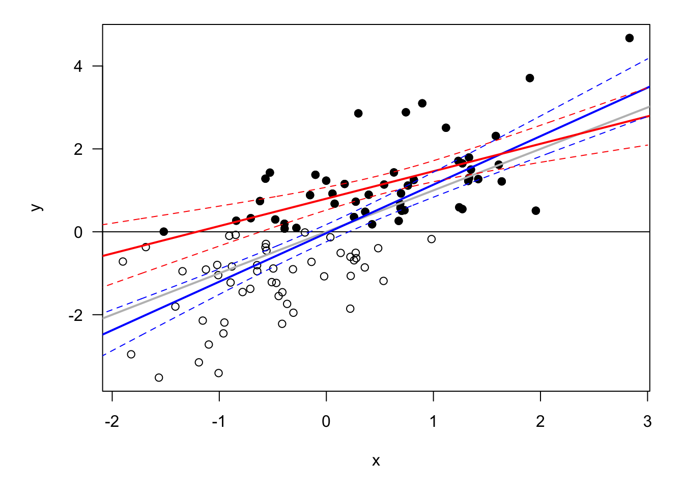
Figure 6.1: Bias in the case of sample selection. The grey line represents the population regression line. The model is \(y_i = x_i + \varepsilon_i\), with \(\varepsilon_{i,t} \sim \mathcal{N}(0,1)\). The red line is the OLS regression line based on black dots only.
Assume that the (partially) observed dependent variable follows: \[ y^* = \boldsymbol\beta'\mathbf{x} + \varepsilon, \] with \(\varepsilon\) is drawn from a distribution characterized by a p.d.f. denoted by \(f_{\boldsymbol\gamma}^*\) and a c.d.f. denoted by \(F_{\boldsymbol\gamma}^*\); these functions depend on a vector of parameters \(\boldsymbol{\gamma}\).
The observed dependent variable is: \[\begin{eqnarray*} \mbox{Censored case:}&&y = \left\{ \begin{array}{ccc} y^* &if& y^*>L \\ L &if& y^*\le L, \end{array} \right.\\ \mbox{Truncated case:}&&y = \left\{ \begin{array}{ccc} y^* &if& y^*>L \\ - &if& y^*\le L, \end{array} \right. \end{eqnarray*}\] where “\(-\)” stands for missing observations.
This formulation is easily extended to censoring from above (\(L \rightarrow U\)), or censoring from both below and above.
The model parameters are gathered in vector \(\theta = [\boldsymbol\beta',\boldsymbol\gamma']'\). Let us write the conditional p.d.f. of the observed variable: \[\begin{eqnarray*} \mbox{Censored case:}&& f(y|\mathbf{x};\theta) = \left\{ \begin{array}{ccc} f_{\boldsymbol\gamma}^*(y - \boldsymbol\beta'\mathbf{x}) &if& y>L \\ F_{\boldsymbol\gamma}^*(L- \boldsymbol\beta'\mathbf{x}) &if& y = L, \end{array} \right.\\ \mbox{Truncated case:}&& f(y|\mathbf{x};\theta) = \dfrac{f_{\boldsymbol\gamma}^*(y - \boldsymbol\beta'\mathbf{x})}{1 - F_{\boldsymbol\gamma}^*(L- \boldsymbol\beta'\mathbf{x})} \quad \mbox{with} \quad y>L. \end{eqnarray*}\]
The (conditional) log-likelihood function is then given by: \[ \log \mathcal{L}(\theta;\mathbf{y},\mathbf{X}) = \sum_{i=1}^n \log f(y_i|\mathbf{x}_i;\theta). \] In the censored case, we have: \[\begin{eqnarray*} \log \mathcal{L}(\theta;\mathbf{y},\mathbf{X}) &=& \sum_{i=1}^n \left\{ \mathbb{I}_{\{y_i=L\}}\log\left[F_{\boldsymbol\gamma}^*(L- \boldsymbol\beta'\mathbf{x}_i)\right] + \right.\\ && \left. \mathbb{I}_{\{y_i>0\}} \log \left[f_{\boldsymbol\gamma}^*(y_i - \boldsymbol\beta'\mathbf{x}_i)\right]\right\}. \end{eqnarray*}\]
The Tobit, or censored/truncated normal regression model, corresponds to the case described above, but with Gaussian errors \(\varepsilon\). Specifically: \[ y^* = \boldsymbol\beta'\mathbf{x} + \varepsilon, \] with \(\varepsilon \sim \,i.i.d.\,\mathcal{N}(0,\sigma^2)\) (\(\Rightarrow\) \(\boldsymbol\gamma = \sigma^2\)).
Without loss of generality, we can assume that \(L=0\). (One can shift observed data if necessary.)
The censored density (with \(L=0\)) is given by: \[ f(y) = \left[ \frac{1}{\sqrt{2 \pi \sigma^2}}\exp\left(-\frac{1}{2 \sigma^2}(y - \boldsymbol\beta'\mathbf{x})^2\right) \right]^{\mathbb{I}_{\{y>0\}}} \left[ 1 - \Phi\left(\frac{\boldsymbol\beta'\mathbf{x}}{\sigma}\right) \right]^{\mathbb{I}_{\{y=0\}}}. \]
The truncated density (with \(L=0\)) is given by: \[ f(y) = \frac{1}{\Phi(\boldsymbol\beta'\mathbf{x})} \frac{1}{\sqrt{2 \pi \sigma^2}}\exp\left(-\frac{1}{2 \sigma^2}(y - \boldsymbol\beta'\mathbf{x})^2\right). \]
Results usually heavily rely on distributional assumptions (more than in uncensored/untruncated case). The framework is easy to extend to an heteroskedastic case, for instance by setting \(\sigma_i^2=\exp(\alpha'\mathbf{x}_i)\). Such a situation is illustrated by Figure 6.2.
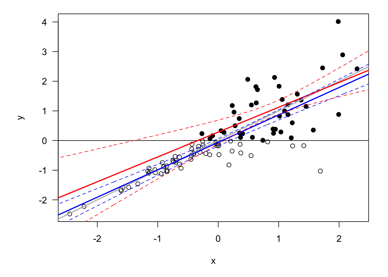
Figure 6.2: Censored dataset with heteroskedasticitiy. The model is \(y_i = x_i + \varepsilon_i\), with \(\varepsilon_{i,t} \sim \mathcal{N}(0,\sigma_i^2)\) where \(\sigma_i = \exp(-1 + x_i)\).
Let us consider the conditional means of \(y\) in the general case, i.e., for any \(\varepsilon\) distribution. Assume \(\mathbf{x}\) is observed, such that expectations are conditional on \(\mathbf{x}\).
For data that are left-truncated at 0, we have: \[\begin{eqnarray*} \mathbb{E}(y) &=& \mathbb{E}(y^*|y^*>0) = \underbrace{\boldsymbol\beta'\mathbf{x}}_{=\mathbb{E}(y^*)} + \underbrace{\mathbb{E}(\varepsilon|\varepsilon>-\boldsymbol\beta'\mathbf{x})}_{>0} > \mathbb{E}(y^*). \end{eqnarray*}\]
Consider data that are left-censored at 0. By Bayes, we have: \[ f_{y^*|y^*>0}(u) = \frac{f_{y^*}(u)}{\mathbb{P}(y^*>0)}\mathbb{I}_{\{u>0\}}. \] Therefore: \[\begin{eqnarray*} \mathbb{E}(y^*|y^*>0) &=& \frac{1}{\mathbb{P}(y^*>0)} \int_{-\infty}^\infty u\, f_{y^*}(u)\mathbb{I}_{\{u>0\}} du \\ &=& \frac{1}{\mathbb{P}(y^*>0)} \mathbb{E}(\underbrace{y^*\mathbb{I}_{\{y^*>0\}}}_{=y}), \end{eqnarray*}\] and, further: \[\begin{eqnarray*} \mathbb{E}(y) &=& \mathbb{P}(y^*>0)\mathbb{E}(y^*|y^*>0)\\ &>& \mathbb{E}(y^*) = \mathbb{P}(y^*>0)\mathbb{E}(y^*|y^*>0) + \mathbb{P}(y^*<0)\underbrace{\mathbb{E}(y^*|y^*<0)}_{<0}. \end{eqnarray*}\]
Now, let us come back to the Tobit (i.e., Gaussian case) case.
For data that are left-truncated at 0: \[\begin{eqnarray} \mathbb{E}(y) &=& \boldsymbol\beta'\mathbf{x} + \mathbb{E}(\varepsilon|\varepsilon>-\boldsymbol\beta'\mathbf{x}) \nonumber\\ &=& \boldsymbol\beta'\mathbf{x} + \sigma \underbrace{\frac{\phi(\boldsymbol\beta'\mathbf{x}/\sigma)}{\Phi(\boldsymbol\beta'\mathbf{x}/\sigma)}}_{=: \lambda(\boldsymbol\beta'\mathbf{x}/\sigma)} = \sigma \left( \frac{\boldsymbol\beta'\mathbf{x}}{\sigma} + \lambda\left(\frac{\boldsymbol\beta'\mathbf{x}}{\sigma}\right)\right). \tag{6.1} \end{eqnarray}\] where the penultimate line is obtained by using Eq. (8.4).
For data that are left-censored at 0: \[\begin{eqnarray*} \mathbb{E}(y) &=& \mathbb{P}(y^*>0)\mathbb{E}(y^*|y^*>0)\\ &=& \Phi\left( \frac{\boldsymbol\beta'\mathbf{x}}{\sigma}\right) \sigma \left( \frac{\boldsymbol\beta'\mathbf{x}}{\sigma} + \lambda\left(\frac{\boldsymbol\beta'\mathbf{x}}{\sigma}\right) \right). \end{eqnarray*}\]
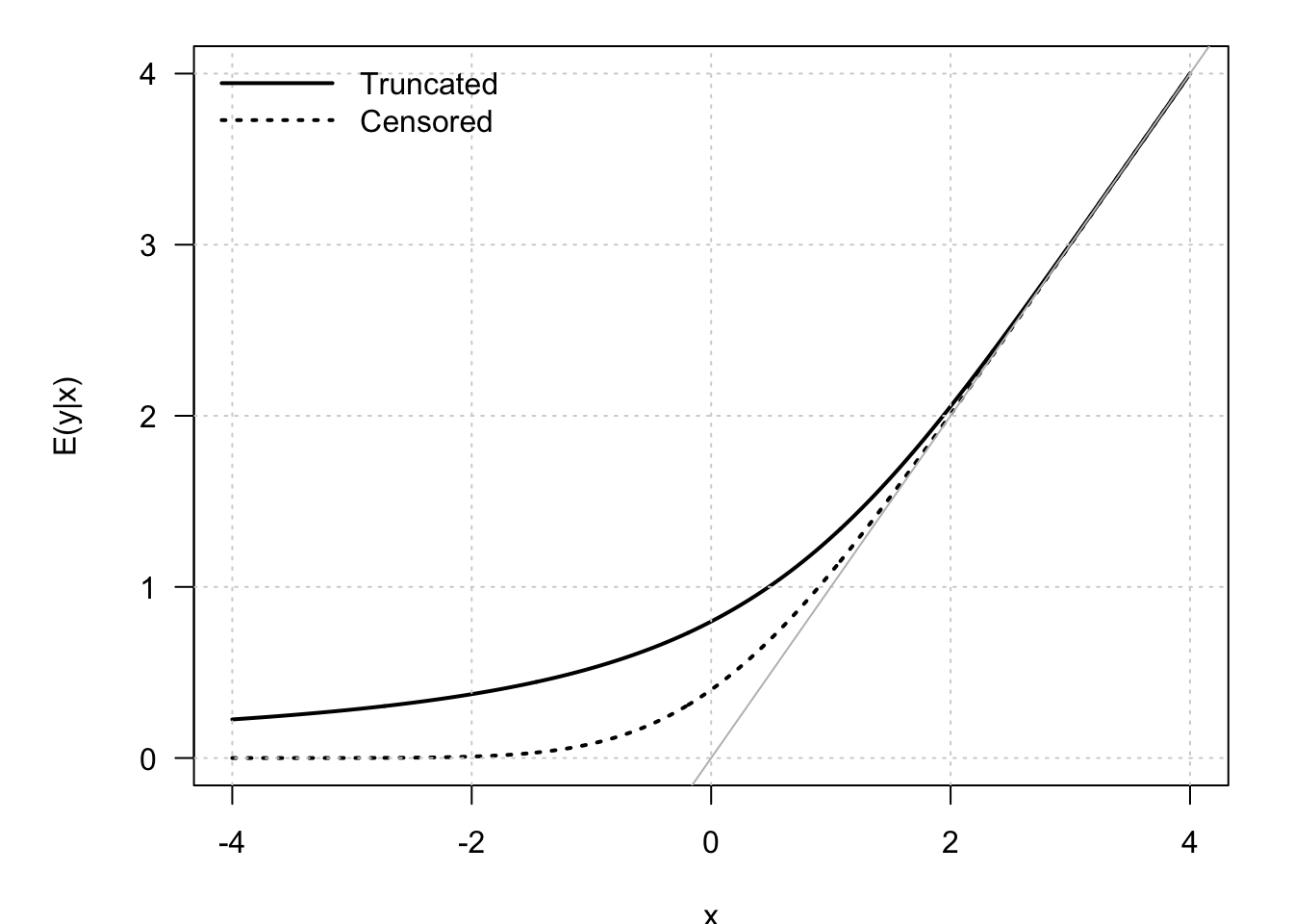
Figure 6.3: Conditional means of \(y\) in Tobit models. The model is \(y_i = x_i + \varepsilon_i\), with \(\varepsilon_i \sim \mathcal{N}(0,1)\).
Heckit regression
The previous formula (Eq. (6.1)) can in particular be used in an alternative estimation approach, namely the Heckman two-step estimation. This approach is based on two steps:16
Using the complete sample, fit a Probit model of \(\mathbb{I}_{\{y_i>0\}}\) on \(\mathbf{x}\). This provides a consistent estimate of \(\frac{\boldsymbol\beta}{\sigma}\), and therefore of \(\lambda(\boldsymbol\beta'\mathbf{x}/\sigma)\). (Indeed, if \(z_i \equiv \mathbb{I}_{\{y_i>0\}}\), then \(\mathbb{P}(z_i=1|\mathbf{x}_i;\boldsymbol\beta/\sigma)=\Phi(\boldsymbol\beta'\mathbf{x}_i/\sigma)\).)
Using the truncated sample only: run an OLS regression of \(\mathbf{y}\) on \(\left\{\mathbf{x},\lambda(\boldsymbol\beta'\mathbf{x}/\sigma)\right\}\) (having Eq. (6.1) in mind). This provides a consistent estimate of \((\boldsymbol\beta,\sigma)\).
The underlying specification is of the form: \[ \mbox{Conditional mean} + \mbox{disturbance}. \] where “Conditional mean” comes from Eq. (6.1) and “disturbance” is an error with zero conditional mean.
This approach is also applied to the case of sample selection models (Section 6.2).
Example 6.1 (Wage prediction) The present example is based on the dataset used in Mroz (1987) (whicht is part of the sampleSelection package).
library(sampleSelection)
library(AER)
data("Mroz87")
Mroz87$lfp.yesno <- NaN
Mroz87$lfp.yesno[Mroz87$lfp==1] <- "yes"
Mroz87$lfp.yesno[Mroz87$lfp==0] <- "no"
Mroz87$lfp.yesno <- as.factor(Mroz87$lfp.yesno)
ols <- lm(wage ~ educ + exper + I( exper^2 ) + city,data=subset(Mroz87,lfp==1))
tobit <- tobit(wage ~ educ + exper + I( exper^2 ) + city,
               left = 0, right = Inf,
               data=Mroz87)
Heckit <- heckit(lfp ~ educ + exper + I( exper^2 ) + city, # selection equation
                 wage ~ educ + exper + I( exper^2 ) + city, # outcome equation
                 data=Mroz87 )

stargazer(ols,Heckit,tobit,no.space = TRUE,type="text",omit.stat = "f")
##
## ======================================================================
## Dependent variable:
## --------------------------------------------------
## wage
## OLS Heckman Tobit
## selection
## (1) (2) (3)
## ----------------------------------------------------------------------
## educ 0.481*** 0.759*** 0.642***
## (0.067) (0.270) (0.081)
## exper 0.032 0.430 0.461***
## (0.062) (0.369) (0.068)
## I(exper2) -0.0003 -0.008 -0.009***
## (0.002) (0.008) (0.002)
## city 0.449 0.113 -0.087
## (0.318) (0.522) (0.378)
## Constant -2.561*** -12.251 -10.395***
## (0.929) (8.853) (1.095)
## ----------------------------------------------------------------------
## Observations 428 753 753
## R2 0.125 0.128
## Adjusted R2 0.117 0.117
## Log Likelihood -1,462.700
## rho 1.063
## Inverse Mills Ratio 5.165 (4.594)
## Residual Std. Error 3.111 (df = 423)
## Wald Test 153.892*** (df = 4)
## ======================================================================
## Note: *p<0.1; **p<0.05; ***p<0.01Figure 6.4 shows that, low wages, the OLS model tends to over-predict wages. The slope between observed and Tobit-predicted wages is closer to one (the adjustment line is closer to the 45-degree line.)
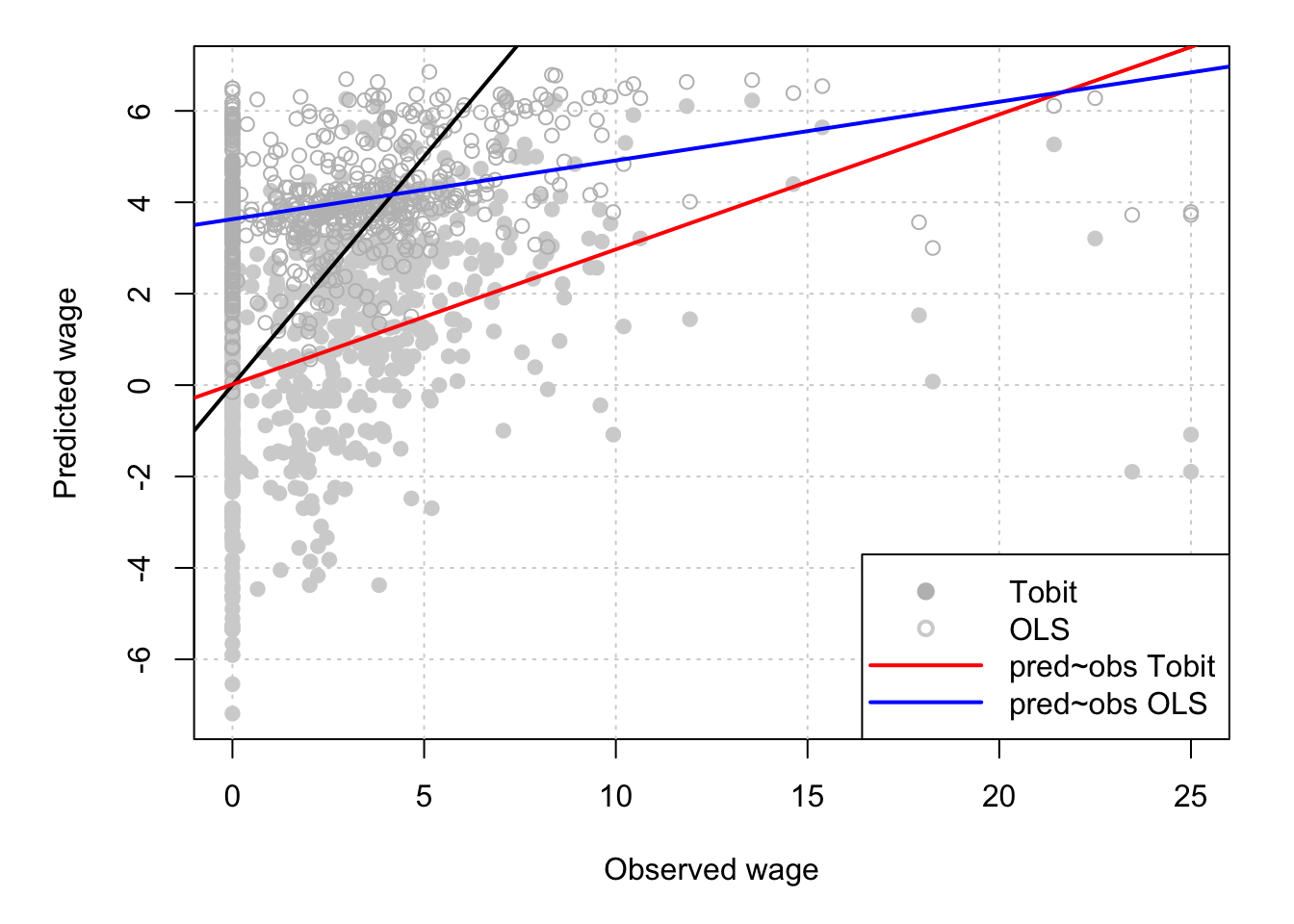
Figure 6.4: Predicted versus observed wages.
Two-part model
In the standard Tobit framework, the model determining censored —or truncated— data censoring mechanism is the same as the one determining non-censored —or observed— data outcome mechanism. A two-part model adds flexibility by permitting the zeros and non-zeros to be generated by different densities. The second model characterizes the outcome conditional on the outcome being observed.
In a seminal paper, Duan et al. (1983) employ this methodology to account for individual annual hospital expenses. The two models are then as follows:
- \(1^{st}\) model: \(\mathbb{P}(hosp=1|\mathbf{x}) = \Phi(\mathbf{x}_1'\boldsymbol\beta_1)\),
- \(2^{nd}\) model: \(Expense = \exp(\mathbf{x}_2'\boldsymbol\beta_2 + \eta)\), with \(\eta \sim\,i.i.d.\, \mathcal{N}(0,\sigma_2^2)\).
Specifically: \[ \mathbb{E}(Expense|\mathbf{x}_1,\mathbf{x}_2) = \Phi(\mathbf{x}_1'\boldsymbol\beta_1)\exp\left(\mathbf{x}_2'\boldsymbol\beta_2+ \frac{\sigma_2^2}{2}\right). \]
In sample-selection models, studied in the next section, one specifies the joint distribution for the censoring and outcome mechanisms (while the two parts are independent here).
6.2 Sample Selection Models
The situation tackled by sample-selection models is the following. The dependent variable of interest, denoted by \(y_2\), depends on observed variables \(\mathbf{x}_2\). Observing \(y_2\), or not, depends on the value of a latent variable (\(y_1^*\)) that is correlated to observed variables \(\mathbf{x}_1\). The difference w.r.t. the two-part model skethed above is that, even conditionally on \((\mathbf{x}_1,\mathbf{x}_2)\), \(y_1^*\) and \(y_2\) may be correlated.
As in the Tobit case, even in the simplest case of population conditional mean linear in regressors (i.e. \(y_2 = \mathbf{x}_2'\boldsymbol\beta_2 + \varepsilon_2\)), OLS regression leads to inconsistent parameter estimates because the sample is not representative of the population.
There are two latent variables: \(y_1^*\) and \(y_2^*\). We observe \(y_1\) and, if the considered entity “participates”, we also observe \(y_2\). More specifically: \[\begin{eqnarray*} y_1 &=& \left\{ \begin{array}{ccc} 1 &\mbox{if}& y_1^* > 0 \\ 0 &\mbox{if}& y_1^* \le 0 \end{array} \right. \quad \mbox{(participation equation)}\\ y_2 &=& \left\{ \begin{array}{ccc} y_2^* &\mbox{if}& y_1 = 1 \\ - &\mbox{if}& y_1 = 0 \end{array} \right. \quad \mbox{(outcome equation).} \end{eqnarray*}\]
Moreover: \[\begin{eqnarray*} y_1^* &=& \mathbf{x}_1'\boldsymbol\beta_1 + \varepsilon_1 \\ y_2^* &=& \mathbf{x}_2'\boldsymbol\beta_2 + \varepsilon_2. \end{eqnarray*}\]
Note that the Tobit model (Section 6.1) is the special case where \(y_1^*=y_2^*\).
Usually: \[ \left[\begin{array}{c}\varepsilon_1\\\varepsilon_2\end{array}\right] \sim \mathcal{N}\left(\mathbf{0}, \left[ \begin{array}{cc} 1 & \rho \sigma_2 \\ \rho \sigma_2 & \sigma_2^2 \end{array} \right] \right). \] Let us derive the likelihood associated with this model. We have: \[\begin{eqnarray} f(\underbrace{0}_{=y_1},\underbrace{-}_{=y_2}|\mathbf{x};\theta) &=& \mathbb{P}(y_1^*\le 0) = \Phi(-\mathbf{x}_1'\boldsymbol\beta_1) \tag{6.2}\\ f(1,y_2|\mathbf{x};\theta) &=& f(y_2^*|\mathbf{x};\theta) \mathbb{P}(y_1^*>0|y_2^*,\mathbf{x};\theta) \nonumber \\ &=& \frac{1}{\sigma}\phi\left(\frac{y_2 - \mathbf{x}_2'\boldsymbol\beta_2}{\sigma}\right) \mathbb{P}(y_1^*>0|y_2,\mathbf{x};\theta).\tag{6.3} \end{eqnarray}\]
Let us compute \(\mathbb{P}(y_1^*>0|y_2,\mathbf{x};\theta)\). By Prop. 8.16 (in Appendix 8.3), applied to (\(\varepsilon_1,\varepsilon_2\)), we have: \[ y_1^*|y_2 \sim \mathcal{N}\left(\mathbf{x}_1'\boldsymbol\beta_1 + \frac{\rho}{\sigma_2}(y_2-\mathbf{x}_2'\boldsymbol\beta_2),1-\rho^2\right). \] which leads to \[\begin{equation} \mathbb{P}(y_1^*>0|y_2,\mathbf{x};\theta) = \Phi\left( \frac{\mathbf{x}_1'\boldsymbol\beta_1 + \dfrac{\rho}{\sigma_2}(y_2-\mathbf{x}_2'\boldsymbol\beta_2)}{\sqrt{1-\rho^2}}\right).\tag{6.4} \end{equation}\]
Figure 6.5 displays \(\mathbb{P}(y_1^*>0|y_2,\mathbf{x};\theta)\) for different values of \(y_2\) and of \(\rho\), in the case where \(\boldsymbol\beta_1=\boldsymbol\beta_2=0\).
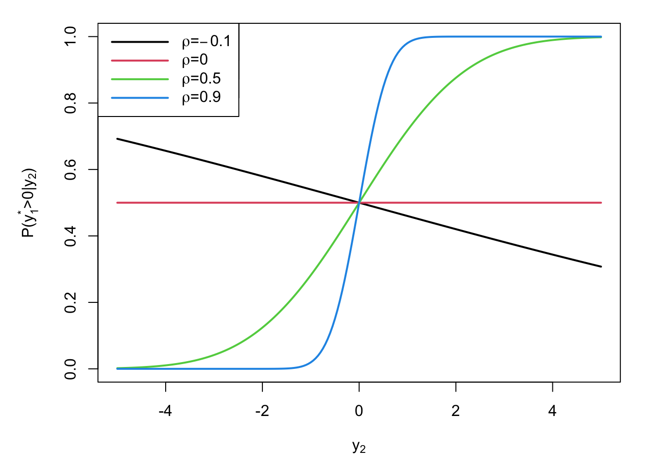
Figure 6.5: Probability of observing \(y_2\) depending on its value, for different values of conditional correlation between \(y_2\) and \(y_1^*\).
Using Eqs. (6.2), (6.3) and (6.4), one gets the log-likelihood function: \[\begin{eqnarray*} \log \mathcal{L}(\theta;\mathbf{y},\mathbf{X}) &=& \sum_{i=1}^n (1 - y_{1,i})\log \Phi(-\mathbf{x}_{1,i}'\boldsymbol\beta_1) + \\ && \sum_{i=1}^n y_{1,i} \log \left( \frac{1}{\sigma}\phi\left(\frac{y_{2,i} - \mathbf{x}_{2,i}'\boldsymbol\beta_2}{\sigma}\right)\right) + \\ && \sum_{i=1}^n y_{1,i} \log \left(\Phi\left( \frac{\mathbf{x}_{1,i}'\boldsymbol\beta_1 + \dfrac{\rho}{\sigma_2}(y_{2,i}-\mathbf{x}_2'\boldsymbol\beta_2)}{\sqrt{1-\rho^2}}\right)\right). \end{eqnarray*}\]
We can also compute conditional expectations: \[\begin{eqnarray} \mathbb{E}(y_2^*|y_1=1,\mathbf{x}) &=& \mathbb{E}(\mathbb{E}(y_2^*|y_1^*,\mathbf{x})|y_1=1,\mathbf{x})\nonumber\\ &=& \mathbb{E}(\mathbf{x}_2'\boldsymbol\beta_2 + \rho\sigma_2(y_1^*-\mathbf{x}_1'\boldsymbol\beta_1)|y_1=1,\mathbf{x})\nonumber\\ &=& \mathbf{x}_2'\boldsymbol\beta_2 + \rho\sigma_2\mathbb{E}( \underbrace{y_1^*-\mathbf{x}_1'\boldsymbol\beta_1}_{=\varepsilon_1 \sim\mathcal{N}(0,1)}|\varepsilon_1>-\mathbf{x}_1'\boldsymbol\beta_1,\mathbf{x})\nonumber\\ &=& \mathbf{x}_2'\boldsymbol\beta_2 + \rho\sigma_2\frac{\phi(-\mathbf{x}_1'\boldsymbol\beta_1)}{1 - \Phi(-\mathbf{x}_1'\boldsymbol\beta_1)}\nonumber\\ &=& \mathbf{x}_2'\boldsymbol\beta_2 + \rho\sigma_2\frac{\phi(\mathbf{x}_1'\boldsymbol\beta_1)}{\Phi(\mathbf{x}_1'\boldsymbol\beta_1)}=\mathbf{x}_2'\boldsymbol\beta_2 + \rho\sigma_2\lambda(\mathbf{x}_1'\boldsymbol\beta_1),\tag{6.5} \end{eqnarray}\] and: \[\begin{eqnarray*} \mathbb{E}(y_2^*|y_1=0,\mathbf{x}) &=& \mathbf{x}_2'\boldsymbol\beta_2 + \rho\sigma_2\mathbb{E}(y_1^*-\mathbf{x}_1'\boldsymbol\beta_1|\varepsilon_1\le-\mathbf{x}_1'\boldsymbol\beta_1,\mathbf{x})\\ &=& \mathbf{x}_2'\boldsymbol\beta_2 + \rho\sigma_2\frac{\phi(-\mathbf{x}_1'\boldsymbol\beta_1)}{1 - \Phi(-\mathbf{x}_1'\boldsymbol\beta_1)}\\ &=& \mathbf{x}_2'\boldsymbol\beta_2 - \rho\sigma_2\frac{\phi(-\mathbf{x}_1'\boldsymbol\beta_1)}{\Phi(-\mathbf{x}_1'\boldsymbol\beta_1)}=\mathbf{x}_2'\boldsymbol\beta_2 - \rho\sigma_2\lambda(-\mathbf{x}_1'\boldsymbol\beta_1). \end{eqnarray*}\]
Heckman procedure
As for tobit models (Section 6.1), we can use the Heckman procedure to estimate this model. Eq. (6.5) shows that \(\mathbb{E}(y_2^*|y_1=1,\mathbf{x}) \ne \mathbf{x}_2'\boldsymbol\beta_2\) when \(\rho \ne 0\). Therefore, the OLS approach yields biased estimates based when it is employed only on the sub-sample where \(y_1=1\).
The Heckman two-step procedure (or “Heckit”) consists in replacing \(\lambda(\mathbf{x}_1'\boldsymbol\beta_1)\) appearing in Eq. (6.5) with a consistent estimate of it. More precisely:
- Get an estimate \(\widehat{\boldsymbol\beta_1}\) of \(\boldsymbol\beta_1\) (probit regression of \(y_1\) on \(\mathbf{x}_1\)).
- Run the OLS regression (using only data associated with \(y_1=1\)): \(\lambda(\mathbf{x}_1'\widehat{\boldsymbol\beta_1})\) as a regressor.
How to estimate \(\sigma_2^2\)? By Eq. (8.5), we have: \[ \mathbb{V}ar(y_2|y_1^*>0,\mathbf{x}) = \mathbb{V}ar(\varepsilon_2|\varepsilon_1>-\mathbf{x}_1'\boldsymbol\beta_1,\mathbf{x}). \] Using that \(\varepsilon_2\) can be decomposed as \(\rho\sigma_2\varepsilon_1 + \xi\), where \(\xi \sim \mathcal{N}(0,\sigma_2^2(1-\rho^2))\) is independent from \(\varepsilon_1\), we get: \[ \mathbb{V}ar(y_2|y_1^*>0,\mathbf{x}) = \sigma_2^2(1-\rho^2) + \rho^2\sigma_2^2 \mathbb{V}ar(\varepsilon_1|\varepsilon_1>-\mathbf{x}_1'\boldsymbol\beta_1,\mathbf{x}). \] Using Eq. (8.6), we get: \[ \mathbb{V}ar(\varepsilon_1|\varepsilon_1>-\mathbf{x}_1'\boldsymbol\beta_1,\mathbf{x}) = 1 - \mathbf{x}_1'\boldsymbol\beta_1 \lambda(\mathbf{x}_1'\boldsymbol\beta_1) - \lambda(\mathbf{x}_1'\boldsymbol\beta_1)^2, \] which gives \[\begin{eqnarray*} \mathbb{V}ar(y_2|y_1^*>0,\mathbf{x}) &=& \sigma_2^2(1-\rho^2) + \rho^2\sigma_2^2 (1 - \mathbf{x}_1'\boldsymbol\beta_1 \lambda(\mathbf{x}_1'\boldsymbol\beta_1) - \lambda(\mathbf{x}_1'\boldsymbol\beta_1)^2)\\ &=& \sigma_2^2 - \rho^2\sigma_2^2 \left(\mathbf{x}_1'\boldsymbol\beta_1 \lambda(\mathbf{x}_1'\boldsymbol\beta_1) + \lambda(\mathbf{x}_1'\boldsymbol\beta_1)^2\right), \end{eqnarray*}\] and, finally: \[ \sigma_2^2 \approx \widehat{\mathbb{V}ar}(y_2|y_1^*>0,\mathbf{x}) + \widehat{\rho \sigma_2}^2 \left(\mathbf{x}_1'\widehat{\boldsymbol\beta_1} \lambda(\mathbf{x}_1'\widehat{\boldsymbol\beta_1}) + \lambda(\mathbf{x}_1'\widehat{\boldsymbol\beta_1})^2\right). \]
The Heckman procedure is computationally simple. Although computational costs are no longer an issue, the two-step solution allows certain generalisations more easily than ML, and is more robust in certain circumstances. The computation of parameter standard errors is fairly complicated because of the two steps (see Cameron and Trivedi (2005), Subsection 16.10.2). Bootstrap can be resorted to.
Example 6.2 (Wage prediction) As in Example 6.1, let us use the Mroz (1987) dataset again, with the objective of explaining wage setting.
library(sampleSelection)
library(AER)
data("Mroz87")
Mroz87$lfp.yesno <- NaN
Mroz87$lfp.yesno[Mroz87$lfp==1] <- "yes"
Mroz87$lfp.yesno[Mroz87$lfp==0] <- "no"
Mroz87$lfp.yesno <- as.factor(Mroz87$lfp.yesno)
#Logit & Probit (selection equation)
logitW <- glm(lfp ~ age + I( age^2 ) + kids5 + huswage + educ,
              family = binomial(link = "logit"), data = Mroz87)
probitW <- glm(lfp ~ age + I( age^2 ) + kids5 + huswage + educ,
               family = binomial(link = "probit"), data = Mroz87)
# OLS for outcome:
ols1 <- lm(log(wage) ~ educ+exper+I( exper^2 )+city,data=subset(Mroz87,lfp==1))
# Two-step Heckman estimation
heckvan <-
  heckit( lfp ~ age + I( age^2 ) + kids5 + huswage + educ, # selection equation
          log(wage) ~ educ + exper + I( exper^2 ) + city, # outcome equation
          data=Mroz87 )
# Maximun likelihood estimation of selection model:
ml <- selection(lfp~age+I(age^2)+kids5+huswage+educ,
                log(wage)~educ+exper+I(exper^2)+city, data = Mroz87)
# Print selection-equation estimates:
stargazer(logitW,probitW,heckvan,ml,type = "text",no.space = TRUE,
          selection.equation = TRUE)
##
## ===================================================================
## Dependent variable:
## -----------------------------------------------
## lfp
## logistic probit Heckman selection
## selection
## (1) (2) (3) (4)
## -------------------------------------------------------------------
## age 0.012 0.010 0.010 0.010
## (0.114) (0.069) (0.069) (0.069)
## I(age2) -0.001 -0.0005 -0.0005 -0.0005
## (0.001) (0.001) (0.001) (0.001)
## kids5 -1.409*** -0.855*** -0.855*** -0.854***
## (0.198) (0.116) (0.115) (0.116)
## huswage -0.069*** -0.042*** -0.042*** -0.042***
## (0.020) (0.012) (0.012) (0.013)
## educ 0.244*** 0.148*** 0.148*** 0.148***
## (0.040) (0.024) (0.023) (0.024)
## Constant -0.938 -0.620 -0.620 -0.615
## (2.508) (1.506) (1.516) (1.518)
## -------------------------------------------------------------------
## Observations 753 753 753 753
## R2 0.158
## Adjusted R2 0.148
## Log Likelihood -459.955 -459.901 -891.177
## Akaike Inf. Crit. 931.910 931.802
## rho 0.018 0.014 (0.203)
## Inverse Mills Ratio 0.012 (0.152)
## ===================================================================
## Note: *p<0.1; **p<0.05; ***p<0.01
# Print outcome-equation estimates:
stargazer(ols1,heckvan,ml,type = "text",no.space = TRUE,omit.stat = "f")
##
## ================================================================
## Dependent variable:
## --------------------------------------------
## log(wage)
## OLS Heckman selection
## selection
## (1) (2) (3)
## ----------------------------------------------------------------
## educ 0.106*** 0.106*** 0.106***
## (0.014) (0.017) (0.017)
## exper 0.041*** 0.041*** 0.041***
## (0.013) (0.013) (0.013)
## I(exper2) -0.001** -0.001** -0.001**
## (0.0004) (0.0004) (0.0004)
## city 0.054 0.053 0.053
## (0.068) (0.069) (0.069)
## Constant -0.531*** -0.547* -0.544**
## (0.199) (0.289) (0.272)
## ----------------------------------------------------------------
## Observations 428 753 753
## R2 0.158 0.158
## Adjusted R2 0.150 0.148
## Log Likelihood -891.177
## rho 0.018 0.014 (0.203)
## Inverse Mills Ratio 0.012 (0.152)
## Residual Std. Error 0.667 (df = 423)
## ================================================================
## Note: *p<0.1; **p<0.05; ***p<0.01